Querying Social Graphs

An example of querying a social graph with Kinetica (no external dataset required)

Prerequisites

The prerequisites for running the query graph example are listed below:

Graph server enabled
Python API
Query graph script

Python API Installation

The native Kinetica Python API is accessible through the following means:

PyPI
Git

PyPI

The Python package manager, pip, is required to install the API from PyPI.

Install the API:
1

pip install gpudb --upgrade
Test the installation:
1

python -c "import gpudb;print('Import Successful')"
If Import Successful is displayed, the API has been installed as is ready for use.

Git

In the desired directory, run the following, but be sure to replace <kinetica-version> with the name of the installed Kinetica version, e.g., v7.1:
1

git clone -b release/<kinetica-version> --single-branch https://github.com/kineticadb/kinetica-api-python.git
Change directory into the newly downloaded repository:
1

cd kinetica-api-python
In the root directory of the unzipped repository, install the Kinetica API:
1

sudo python setup.py install
Test the installation (Python 2.7 (or greater) is necessary for running the API example):
1

python examples/example.py

Script Detail

This example is going to demonstrate querying a social network of relationships between friends and family for:

people directly or indirectly known to a given person who are interested in chess but not known through family
people directly known to a given gender
people who are of a given gender or interested in chess
people directly or indirectly known to a given gender who are interested in chess

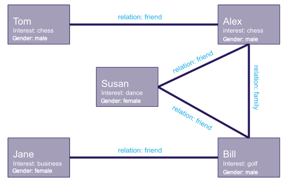
The graph queried in the examples below looks like this:

Constants

Several constants are defined at the beginning of the script:

SCHEMA -- the name of the schema in which the tables supporting the graph creation and match operations will be created

Important

The schema is created during the table setup portion of the script because the schema must exist prior to creating the tables that will later support the graph creation and match operations.
TABLE_P / TABLE_K -- the names for the tables into which the datasets generated in this file are loaded. These datasets will serve as the basis for the social relationships graph. TABLE_P is a record of a person's name, age, and interest; TABLE_K defines the relationships between the people
GRAPH_S -- the social relationships graph
TABLE_Q1 / TABLE_Q2 / TABLE_Q3 / TABLE_Q4 -- the resulting adjacency tables from the four query examples performed in the script
TABLE_Q1_TARGETS / TABLE_Q2_TARGETS / TABLE_Q3_TARGETS / TABLE_Q4_TARGETS-- the table storing the targets from the first query

Constant Definitions



 1
 2
 3
 4
 5
 6
 7
 8
 9
10
11
12
13


SCHEMA = "graph_q_social"
TABLE_P = SCHEMA + ".people"
TABLE_K = SCHEMA + ".knows"

GRAPH_S = SCHEMA + "." + "social_relationships"
TABLE_Q1 = GRAPH_S + "_queried_jane_to_chess"
TABLE_Q2 = GRAPH_S + "_queried_males"
TABLE_Q3 = GRAPH_S + "_queried_females_or_chess"
TABLE_Q4 = GRAPH_S + "_queried_females_to_chess"
TABLE_Q1_TARGETS = TABLE_Q1 + "_nodes"
TABLE_Q2_TARGETS = TABLE_Q2 + "_nodes"
TABLE_Q3_TARGETS = TABLE_Q3 + "_nodes"
TABLE_Q4_TARGETS = TABLE_Q4 + "_nodes"

Table Setup

As mentioned previously, there are two tables used in the graph creation step. The first of these tables is the people table. It is created using the GPUdbTable interface:

Create People Table



 1
 2
 3
 4
 5
 6
 7
 8
 9
10
11


table_p_obj = gpudb.GPUdbTable(
    _type = [
        ["name", "string", "char16"],
        ["age", "int"],
        ["interest", "string", "char16"],
        ["gender", "string", "char8"]
    ],
    name = TABLE_P,
    db = kinetica,
    options = {}
)

Finally, the people records are defined and inserted:

Populate People Table



1
2
3
4
5
6
7
8


p_records = [
    ["Susan", 22, "dance", "female"],
    ["Bill", 60, "golf", "male"],
    ["Alex", 34, "chess", "male"],
    ["Jane", 40, "business", "female"],
    ["Tom", 29, "chess", "male"]
]
table_p_obj.insert_records(p_records)

The second table is the knows table. It is also created using the GPUdbTable interface:

Create Relation Table



 1
 2
 3
 4
 5
 6
 7
 8
 9
10
11


table_k_obj = gpudb.GPUdbTable(
    _type = [
        ["name1", "string", "char16"],
        ["name2", "string", "char16"],
        ["since", "long"],
        ["relation", "string", "char32"]
    ],
    name = TABLE_K,
    db = kinetica,
    options = {}
)

Finally, the knows records are defined and inserted:

Populate Relation Table



1
2
3
4
5
6
7
8


k_records = [
    ["Jane", "Bill", 2010, "friend"],
    ["Bill", "Susan", 1990, "friend"],
    ["Bill", "Alex", 2001, "family"],
    ["Alex", "Tom", 2001, "friend"],
    ["Susan", "Alex", 2002, "friend"]
]
table_k_obj.insert_records(k_records)

Graph Creation

Social Graphs

Create social graphs in Kinetica

One graph is used for the query graph example: social_relationships, a graph based on the people and knows datasets.

The social_relationships graph is created with the following characteristics:

It is not directed because relationships between people are inherently bi-directional
The people in this graph are represented using nodes detailed in the people table: the person's (NAME), their main interest (LABEL), and gender (LABEL).
The relationships in this graph are represented using edges detailed in the knows table: two names to define the relationship (NODE1_NAME / NODE2_NAME) and the relationship definition (LABEL).
It has no weights because this example doesn't favor some relationships over others
It has no inherent restrictions for any of the nodes or edges in the graph

Note

Restrictions will be introduced on a per-query basis later.
It will be replaced with this instance of the graph if a graph of the same name exists (recreate)

Create Social Graph



 1
 2
 3
 4
 5
 6
 7
 8
 9
10
11
12
13
14
15
16
17
18
19
20
21


create_s_graph_response = kinetica.create_graph(
    graph_name = GRAPH_S,
    directed_graph = False,
    nodes = [
        TABLE_P + ".name AS NAME",
        TABLE_P + ".interest AS LABEL",
        "",
        TABLE_P + ".name AS NAME",
        TABLE_P + ".gender AS LABEL"
    ],
    edges = [
        TABLE_K + ".name1 AS NODE1_NAME",
        TABLE_K + ".name2 AS NODE2_NAME",
        TABLE_K + ".relation AS LABEL"
    ],
    weights = [],
    restrictions = [],
    options = {
        "recreate": "true"
    }
)

Querying the Graph

Example 1

To find people interested in chess who are connected to a given person, in this case Jane, in some way (but not through family), we define the graph query in the following way:

Pass two query identifiers to queries:
- One using Jane as the name (NODE_NAME) of the node from which to begin searching
- Pass a blank string ("") to separate the first query combination from the second
- The other using chess as the label of the target nodes to find (TARGET_NODE_LABEL)
Use the following restrictions:
- Pass 'family' as the label (EDGE_LABEL) of the edge in the restriction combination
- Pass a 0 as an "off" value (ONOFFCOMPARED) for the edge to set it as restricted
Place the results in social_relationships_queried_jane_chess adjacency table and the targets found in the social_relationships_queried_jane_chess_nodes table
Query for nodes within 4 "hops" (rings) of Jane

Query Graph Example #1



 1
 2
 3
 4
 5
 6
 7
 8
 9
10
11
12
13
14


query1_s_graph_response = kinetica.query_graph(
    graph_name = GRAPH_S,
    queries = [
        "{'Jane'} AS NODE_NAME",
        "",
        "{'chess'} AS TARGET_NODE_LABEL"
    ],
    restrictions = [
        "{'family'} AS EDGE_LABEL",
        "{0} AS ONOFFCOMPARED"
    ],
    adjacency_table = TABLE_Q1,
    rings = 4
)

The results are retrieved from the social_relationships_queried_jane_chess adjacency table. The results show two people connected to Jane that are interested in chess, Alex and Tom. The path to each is listed (represented by PATH_ID) and the hops to get there (represented by RING_ID). Note that the PATH_ID and RING_ID data were only available because the TARGET_NODE_LABEL query identifier was used in the query:

Query Graph Example #1 Adjacencies



 1
 2
 3
 4
 5
 6
 7
 8
 9
10
11
12
13
14
15
16
17


+-----------------+--------------------+--------------------+-----------+-----------+
|   QUERY_EDGE_ID | QUERY_NODE1_NAME   | QUERY_NODE2_NAME   |   PATH_ID |   RING_ID |
+=================+====================+====================+===========+===========+
|               1 | Jane               | Bill               |         2 |         1 |
+-----------------+--------------------+--------------------+-----------+-----------+
|               2 | Bill               | Susan              |         2 |         2 |
+-----------------+--------------------+--------------------+-----------+-----------+
|               5 | Susan              | Alex               |         2 |         3 |
+-----------------+--------------------+--------------------+-----------+-----------+
|               1 | Jane               | Bill               |         3 |         1 |
+-----------------+--------------------+--------------------+-----------+-----------+
|               2 | Bill               | Susan              |         3 |         2 |
+-----------------+--------------------+--------------------+-----------+-----------+
|               5 | Susan              | Alex               |         3 |         3 |
+-----------------+--------------------+--------------------+-----------+-----------+
|               4 | Alex               | Tom                |         3 |         4 |
+-----------------+--------------------+--------------------+-----------+-----------+

The targets are retrieved from the social_relationships_queried_jane_chess_nodes table, which shows the RING_ID, the query sources, and the targets' names, Alex and Tom. The RING_ID represents the hops required to get from the source to the target.

Query Graph Example #1 Targets



1
2
3
4
5
6
7


+------------------------+------------------------+--------------------------+--------------------------+-----------+
|   QUERY_NODE_ID_SOURCE |   QUERY_NODE_ID_TARGET | QUERY_NODE_NAME_SOURCE   | QUERY_NODE_NAME_TARGET   |   RING_ID |
+========================+========================+==========================+==========================+===========+
|                      4 |                      3 | Jane                     | Alex                     |         3 |
+------------------------+------------------------+--------------------------+--------------------------+-----------+
|                      4 |                      5 | Jane                     | Tom                      |         4 |
+------------------------+------------------------+--------------------------+--------------------------+-----------+

Example 2

To find people directly connected to a given gender, in this case male, we define the graph query in the following way:

Pass a single query to queries using male as the label (NODE_LABEL) of the node from which to begin searching
Place the results in social_relationships_queried_males adjacency table and the targets found in the social_relationships_queried_males_nodes table
Use a rings value of 1 to only retrieve immediate connections to males

Query Graph Example #2



1
2
3
4
5
6
7
8
9


query2_s_graph_response = kinetica.query_graph(
    graph_name = GRAPH_S,
    queries = [
        "{'male'} AS NODE_LABEL"
    ],
    restrictions = [],
    adjacency_table = TABLE_Q2,
    rings = 1
)

The results are retrieved from the social_relationships_queried_males adjacency table. The results show each node within one "hop" of a male node:

Query Graph Example #2 Adjacencies



 1
 2
 3
 4
 5
 6
 7
 8
 9
10
11
12
13
14
15
16
17


+-----------------+--------------------+--------------------+
|   QUERY_EDGE_ID | QUERY_NODE1_NAME   | QUERY_NODE2_NAME   |
+=================+====================+====================+
|               1 | Jane               | Bill               |
+-----------------+--------------------+--------------------+
|               2 | Bill               | Susan              |
+-----------------+--------------------+--------------------+
|               3 | Bill               | Alex               |
+-----------------+--------------------+--------------------+
|               3 | Bill               | Alex               |
+-----------------+--------------------+--------------------+
|               4 | Alex               | Tom                |
+-----------------+--------------------+--------------------+
|               4 | Alex               | Tom                |
+-----------------+--------------------+--------------------+
|               5 | Susan              | Alex               |
+-----------------+--------------------+--------------------+

The targets are retrieved from the social_relationships_queried_males_nodes target nodes table. The results show the name for all nodes that are connected to the male nodes within one "hop". Duplicate names indicate that person is within one "hop" of more than one male:

Query Graph Example #2 Targets



 1
 2
 3
 4
 5
 6
 7
 8
 9
10
11
12
13
14
15
16
17


+------------------------+--------------------------+
|   QUERY_NODE_ID_TARGET | QUERY_NODE_NAME_TARGET   |
+========================+==========================+
|                      1 | Susan                    |
+------------------------+--------------------------+
|                      1 | Susan                    |
+------------------------+--------------------------+
|                      2 | Bill                     |
+------------------------+--------------------------+
|                      3 | Alex                     |
+------------------------+--------------------------+
|                      3 | Alex                     |
+------------------------+--------------------------+
|                      4 | Jane                     |
+------------------------+--------------------------+
|                      5 | Tom                      |
+------------------------+--------------------------+

Example 3

To find people who are of a given gender, in this case female, or are interested in chess, we define the graph query in the following way:

Pass a single query to queries using female and chess as the label (NODE_LABEL) of the node for which to search
Place the results in social_relationships_queried_females_or_chess adjacency table and the targets found in the social_relationships_queried_females_or_chess_nodes table
Use a rings value of 0 to only retrieve the nodes that satisfy the query labels

Query Graph Example #3



1
2
3
4
5
6
7
8
9


query3_s_graph_response = kinetica.query_graph(
    graph_name = GRAPH_S,
    queries = [
        "{'female', 'chess'} AS NODE_LABEL",
    ],
    restrictions = [],
    adjacency_table = TABLE_Q3,
    rings = 0
)

There are no results in the social_relationships_queried_females_or_chess because the rings value was set to 0, meaning there will be no adjacencies.

The targets are retrieved from the social_relationships_queried_females_or_chess_nodes target nodes table. The results show the name for the nodes that are female or interested in chess:

Query Graph Example #3 Targets



 1
 2
 3
 4
 5
 6
 7
 8
 9
10
11


+------------------------+--------------------------+
|   QUERY_NODE_ID_TARGET | QUERY_NODE_NAME_TARGET   |
+========================+==========================+
|                      1 | Susan                    |
+------------------------+--------------------------+
|                      3 | Alex                     |
+------------------------+--------------------------+
|                      4 | Jane                     |
+------------------------+--------------------------+
|                      5 | Tom                      |
+------------------------+--------------------------+

Example 4

To find people directly or indirectly known to a given gender who are interested in chess, we define the graph query in the following way:

Pass two query identifiers to queries:
- One using female as the label (NODE_LABEL) of the node from which to begin searching
- Pass a blank string ("") to separate the first query combination from the second
- The other using chess as the label of the target nodes to find (TARGET_NODE_LABEL)
Place the results in social_relationships_queried_females_to_chess adjacency table and the targets found in the social_relationships_queried_females_to_chess_nodes table
Use a rings value of 2 to find nodes within two "hops" of the female nodes

Query Graph Example #4



 1
 2
 3
 4
 5
 6
 7
 8
 9
10
11


query4_s_graph_response = kinetica.query_graph(
    graph_name = GRAPH_S,
    queries = [
        "{'female'} AS NODE_LABEL",
        "",
        "{'chess'} AS TARGET_NODE_LABEL"
    ],
    restrictions = [],
    adjacency_table = TABLE_Q4,
    rings = 2
)

The results are retrieved from the social_relationships_queried_females_to_chess adjacency table. The results show two females, Susan and Jane, connected (within two "hops") to two people that are interested in chess, Alex and Tom. The path to each is listed (represented by PATH_ID) and the hops to get there (represented by RING_ID). Note that the PATH_ID and RING_ID data were only available because the TARGET_NODE_LABEL query identifier was used in the query:

Query Graph Example #4 Adjacencies



 1
 2
 3
 4
 5
 6
 7
 8
 9
10
11
12
13


+-----------------+--------------------+--------------------+-----------+-----------+
|   QUERY_EDGE_ID | QUERY_NODE1_NAME   | QUERY_NODE2_NAME   |   PATH_ID |   RING_ID |
+=================+====================+====================+===========+===========+
|               1 | Jane               | Bill               |         1 |         1 |
+-----------------+--------------------+--------------------+-----------+-----------+
|               3 | Bill               | Alex               |         1 |         2 |
+-----------------+--------------------+--------------------+-----------+-----------+
|               5 | Susan              | Alex               |         3 |         1 |
+-----------------+--------------------+--------------------+-----------+-----------+
|               5 | Susan              | Alex               |         4 |         1 |
+-----------------+--------------------+--------------------+-----------+-----------+
|               4 | Alex               | Tom                |         4 |         2 |
+-----------------+--------------------+--------------------+-----------+-----------+

The targets are retrieved from the social_relationships_queried_females_to_chess_nodes target nodes table. The results show the name for the nodes that are interested in chess and the "hops" required to get there:

Query Graph Example #4 Targets



1
2
3
4
5
6
7
8
9


+------------------------+------------------------+--------------------------+--------------------------+-----------+
|   QUERY_NODE_ID_SOURCE |   QUERY_NODE_ID_TARGET | QUERY_NODE_NAME_SOURCE   | QUERY_NODE_NAME_TARGET   |   RING_ID |
+========================+========================+==========================+==========================+===========+
|                      1 |                      3 | Susan                    | Alex                     |         1 |
+------------------------+------------------------+--------------------------+--------------------------+-----------+
|                      1 |                      5 | Susan                    | Tom                      |         2 |
+------------------------+------------------------+--------------------------+--------------------------+-----------+
|                      4 |                      3 | Jane                     | Alex                     |         2 |
+------------------------+------------------------+--------------------------+--------------------------+-----------+

Download & Run

Included below is a complete example containing all the above requests, the data files, and output.

To run the complete sample, switch to the directory in which the query_graph_social.py is located, then do the following:

Run Example

1

python query_graph_social.py [--url <target_url>] --username <username> --password <password>