Using WKT Data and Geospatial Functions
Learn how to ingest and use WKT geometry with geospatial functions
Learn how to ingest and use WKT geometry with geospatial functions
The following sections demonstrate how to ingest and work with WKT data as well as how to use geospatial functions via SQL and the Kinetica Python API. Details about the geospatial functions can be found under Geospatial/Geometry Functions. All geospatial functions are compatible in both native API and SQL.
Data loading will be done via SQL. First log in to the database:
|
|
Create a schema to house the example tables.
|
|
Create tables for geospatial & temporal data within the schema.
|
|
|
|
|
|
Populate the example tables with source data. The files are staged into KiFS from the directory that is local to where KiSQL is running. From there, each is loaded into its respective table. Modify these statements as necessary to reflect the location of the data files on the client machine.
|
|
|
|
|
|
|
|
|
|
|
|
|
|
First, a points-of-interest table is created and loaded with sample WKT data.
|
|
Then, data is inserted into the WKT table.
|
|
For the complete list of scalar functions, see both Scalar Functions and Enhanced Performance Scalar Functions.
|
|
|
|
For the complete list of aggregation functions, see Aggregation Functions.
|
|
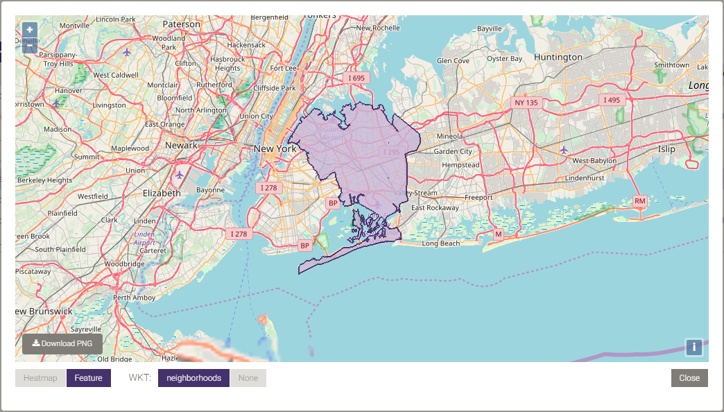
Below is a picture of the dissolved neighborhood boundaries:
Many geospatial/geometry functions can be used to join data sets. For the complete list of join and other scalar functions, see both Scalar Functions and Enhanced Performance Scalar Functions.
|
|
|
|
In some cases, it may be useful to aggregate on the geospatial column itself, applying standard aggregation functions to other joined columns.
|
|
There are three ways of checking if two geometries are equal, which each have different thresholds:
For details on these functions see Scalar Functions.
The data inserted in the first section includes two POINTs that vary slightly in precision, two POLYGONs that vary in the ordering of their boundary points, and two pairs of LINESTRINGs that vary in both precision and scale. Each of these geometry types is compared to see if each given pair is spatially equal as defined by the equality functions:
|
|
First, a points-of-interest table is created and loaded with sample WKT data.
|
|
Then, data is inserted into the WKT table, and the insertion is verified.
|
|
For the complete list of scalar functions, see both Scalar Functions and Enhanced Performance Scalar Functions.
|
|
|
|
For the complete list of aggregation functions, see Aggregation Functions.
|
|
Below is a picture of the dissolved neighborhood boundaries:
Many geospatial/geometry functions can be used to join data sets. For the complete list of join and other scalar functions, see both Scalar Functions and Enhanced Performance Scalar Functions.
|
|
|
|
In some cases, it may be useful to aggregate on the geospatial column itself, applying standard aggregation functions to other joined columns.
|
|
There are three ways of checking if two geometries are equal, which each have different thresholds:
For details on these functions see Scalar Functions.
The data inserted in the first section includes two POINTs that vary slightly in precision, two POLYGONs that vary in the ordering of their boundary points, and two pairs of LINESTRINGs that vary in both precision and scale. Each of these geometry types is compared to see if each given pair is spatially equal as defined by the equality functions:
|
|
Included below are complete examples containing all the above requests and the output.