> ## Documentation Index
> Fetch the complete documentation index at: https://docs.kinetica.com/llms.txt
> Use this file to discover all available pages before exploring further.
# Generate Isochrones
> Learn how to create isochrones with Kinetica's Graph
The following is a complete example, using the *Python API*, of generating
images containing isochrones via the [/visualize/isochrone](/content/api/rest/visualize_isochrone_rest)
and [/wms](/content/api/rest/wms_rest) endpoints using an existing
[graph](/content/graph_solver/network_graph_solver).
## Prerequisites
The prerequisites for running the isochrones example are listed below:
* Graph server enabled
* Python API
* [Isochrones example script](https://raw.githubusercontent.com/kineticadb/kinetica-docs/master/content/examples/python/isochrones.py)
* [DC Shape data CSV file](https://raw.githubusercontent.com/kineticadb/kinetica-docs/master/content/examples/data/dc_shape.csv)
## Python API Installation
Depending on the target operating system, a Python virtual environment may need
to be installed first:
* [Python Virtual Environment](#python-virtual-environment)
The native *Kinetica Python API* is accessible through the following means:
* [PyPI](#pypi)
* [Git](#git)
### Python Virtual Environment
A Python virtual environment is necessary to install in an operating environment
where Python is externally managed.
1. Install a Python virtual environment:
```bash theme={null}
python3 -m venv .venv
```
2. Activate the Python virtual environment:
```bash theme={null}
source .venv/bin/activate
```
### PyPI
1. Install the API:
```bash theme={null}
pip3 install gpudb
```
2. Test the installation:
```python theme={null}
python3 -c "import gpudb;print('Import Successful')"
```
If *Import Successful* is displayed, the API has been installed as is ready
for use.
### Git
1. In the desired directory, run the following, but be sure to replace
`` with the name of the installed Kinetica version,
e.g., `v7.2`:
```bash theme={null}
git clone -b release/ --single-branch https://github.com/kineticadb/kinetica-api-python.git
```
2. Change directory into the newly downloaded repository:
```bash theme={null}
cd kinetica-api-python
```
3. In the root directory of the unzipped repository, install the Kinetica API:
```bash theme={null}
sudo pip3 install .
```
4. Test the installation (*Python3* is necessary for running the API example):
```bash theme={null}
python3 examples/example.py
```
### Data File
The example script references the dc\_shape.csv data file,
mentioned in the [Prerequisites](#prerequisites), in the current local directory, by default.
This directory can specified as a parameter when running the script.
## Script Detail
This example is going to demonstrate the following scenarios using isochrones
either via the [/visualize/isochrone](/content/api/rest/visualize_isochrone_rest) endpoint or the
[/wms](/content/api/rest/wms_rest) endpoint:
* Find the shared area between Dulles International Airport (IAD), Ronald
Reagan Washington National Airport (DCA),and Kinetica HQ by calculating the
isochrones for traveling **to** IAD within 40 minutes, traveling **to**
DCA within 25 minutes, and traveling **from** Kinetica HQ within 10 minutes
and joining the results on the intersection of the isochrones using
[/visualize/isochrone](/content/api/rest/visualize_isochrone_rest)
* Calculating the isochrones for traveling **to** Kinetica HQ within 15 minutes
using [/wms](/content/api/rest/wms_rest)
### Connections
This example will use two connections, one to the database and one to the WMS
endpoint, configured as follows:
```python Database Connection theme={null}
kinetica = gpudb.GPUdb(host = [args.url], username = args.username, password = args.password)
```
```python WMS Endpoint URL theme={null}
WMS_URL = args.url + "/wms"
```
### Constants
Many constants are defined at the beginning of the script:
* `CSV_ROW_SIZE` -- the expected row number for the CSV file
* `OPTION_NO_ERROR` -- reference to a [/clear/table](/content/api/rest/clear_table_rest)
option for ease of use and repeatability
* `OPTION_ISO` -- a *Python* dictionary containing
[/visualize/isochrone](/content/api/rest/visualize_isochrone_rest) `options` key-value
pairs
```python theme={null}
OPTION_ISO = {"concavity_level": "0.2", "is_replicated": "true"}
```
* `OPTION_ISO_CONTOUR` -- a *Python* dictionary containing
[/visualize/isochrone](/content/api/rest/visualize_isochrone_rest) `contour_options` key-value
pairs
```python theme={null}
OPTION_ISO_CONTOUR = {
"adjust_grid": "false",
"adjust_levels": "false",
"gridding_method": "INV_DST_POW",
"labels_font_size": "16",
"labels_font_family": "Sans",
"labels_search_window": "4",
"grid_size": str(100),
"min_grid_size": "10",
"max_grid_size": "300",
"search_radius": "9",
"smoothing_factor": "0.000001",
"color_isolines": "true",
"width": "512", "height": "-1"
}
```
* `OPTIONS_ISO_STYLE` -- a *Python* dictionary containing
[/visualize/isochrone](/content/api/rest/visualize_isochrone_rest) `style_options` key-value
pairs
```python theme={null}
OPTION_ISO_STYLE = {
"line_size": "2",
"color": "0xFF000000",
"bg_color": "0x00000000",
"colormap": "jet",
"text_color": "0xFF000000"
}
```
* `SCHEMA` -- the name of the schema in which the tables will be created
* `TABLE_DC` -- the name of the table into which the DC Shape dataset is
loaded
* `TABLE_D_LVL` -- the name of the table into which the IAD isochrone
contour levels are output
* `TABLE_JOIN` -- the name of the *join view* hosting the shared area between
the three isochrone contour level output tables
* `TABLE_K_ISO_SOLVE` -- the name of the table into which the WMS examples'
isochrones solution (the position and cost for each vertex in the underlying
graph) is output
* `TABLE_K_LVL1` -- the name of the table into which the Kinetica isochrone
(leading **from**) contour levels are output
* `TABLE_K_LVL2` -- the name of the table into which the Kinetica isochrone
(leading **to**) contour levels are output
* `TABLE_R_LVL` -- the name of the table into which the DCA isochrone
contour levels are output
* `GRAPH_DC` -- the underlying DC shape graph that powers the isochrone
calculation
* `D_AIR`, `K_HQ`, `R_AIR` -- the source nodes for the IAD, Kinetica HQ, &
DCA isochrone requests,
respectively
```python theme={null}
D_AIR = "POINT(-77.446831 38.955309)"
K_HQ = "POINT(-77.115203 38.881578)"
R_AIR = "POINT(-77.042295 38.849684)"
```
* `D_AIR_IMG`, `K_HQ_IMG1`, `K_HQ_IMG2`, `R_AIR_IMG` -- the resulting
generated isochrone image from the IAD, Kinetica HQ (leading **from**),
Kinetica HQ (leading **to**), & DCA isochrone requests, respectively
### Graph Creation
One graph is used for the isochrones examples utilized in the script:
`dc_shape_graph`, a graph based on the `dc_shape` dataset (the CSV file
mentioned in [Prerequisites](#prerequisites)).
The example script will first check to see if the `dc_shape` table
and `dc_shape_graph` exist; if either does not, they will be
created.
The `dc_shape_graph` is created with the following characteristics:
* It is [directed](/content/graph_solver/network_graph_solver#directed-graphs) because the roads in the graph have
directionality (one-way and two-way roads)
* It has no explicitly defined `nodes` because the nodes are not used in these
examples
* The `edges` are represented using WKT LINESTRINGs in the `shape` column
of the `dc_shape` table (`WKTLINE`). Each edge's directionality is
derived from the `direction` column of the `dc_shape`
table (`DIRECTION`).
* The `weights` represent the time taken to travel the edge, which
is derived from the length of the edge divided by the `speed` column values
also found in the `dc_shape` table. This derived time value is mapped to the
`VALUESPECIFIED` [identifier](/content/graph_solver/network_graph_solver#identifiers).
* It has no inherent `restrictions` for any of the nodes or edges in the graph
* It will be replaced with this instance of the graph if a graph of the same
name exists (`recreate`)
```python Create Graph theme={null}
create_graph_dc_resp = kinetica.create_graph(
graph_name = GRAPH_DC,
directed_graph = True,
nodes = [],
edges = [
TABLE_DC + ".direction AS DIRECTION",
TABLE_DC + ".shape AS WKTLINE"
],
weights = [
TABLE_DC + ".direction AS EDGE_DIRECTION",
TABLE_DC + ".shape AS EDGE_WKTLINE",
"ST_LENGTH(" + TABLE_DC + ".shape,1)/" + TABLE_DC + ".speed AS VALUESPECIFIED"
],
restrictions = [],
options = {"recreate": "true"}
)
```
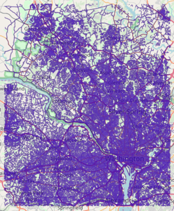
The graph output to WMS:
 ### Visualizing Isochrones
First, additional contour and isochrones options are provided:
* `add_labels` is set to `true` to display labels on the isochrones image
* `projection` is set to `web_mercator` to change the spatial reference
system
* `solve_direction` is set to `to_source` to calculate isochrones leading
**to** IAD
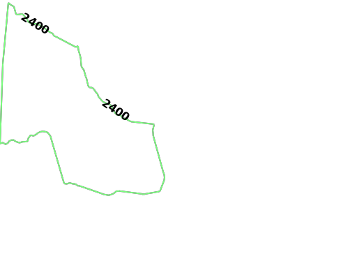
Then, the first group of isochrones is calculated using the following
parameters and an image is generated using
[/visualize/isochrone](/content/api/rest/visualize_isochrone_rest) endpoint:
* `source_node` is provided as a WKT point (`D_AIR`) paired with a
`NODE_WKTPOINT` [identifier](/content/graph_solver/network_graph_solver#identifiers)
* `max_solution_radius` is set for 2400 seconds' (or 40 minutes') worth of
travel surrounding the source node
* `num_levels` is set to `1` to only display one isochrone contour around
the source node
* `generate_image` is set to `True` to generate an image and output it to
the response
```python Request IAD Isochrone Image theme={null}
vis_isochrone_d_resp = kinetica.visualize_isochrone(
graph_name = GRAPH_DC,
source_node = D_AIR + " AS NODE_WKTPOINT",
max_solution_radius = 40 * 60,
num_levels = 1,
generate_image = True,
levels_table = TABLE_D_LVL,
style_options = OPTION_ISO_STYLE,
contour_options = OPTION_ISO_CONTOUR,
options = OPTION_ISO
)
```
The image is pulled from the response and written locally:
```python Write IAD Isochrone Image to Disk theme={null}
img = vis_isochrone_d_resp["image_data"]
img_isochrones_to_dulles = open(D_AIR_IMG, "wb")
img_isochrones_to_dulles.write(img)
img_isochrones_to_dulles.close()
```
The generated image for IAD isochrones:
### Visualizing Isochrones
First, additional contour and isochrones options are provided:
* `add_labels` is set to `true` to display labels on the isochrones image
* `projection` is set to `web_mercator` to change the spatial reference
system
* `solve_direction` is set to `to_source` to calculate isochrones leading
**to** IAD
Then, the first group of isochrones is calculated using the following
parameters and an image is generated using
[/visualize/isochrone](/content/api/rest/visualize_isochrone_rest) endpoint:
* `source_node` is provided as a WKT point (`D_AIR`) paired with a
`NODE_WKTPOINT` [identifier](/content/graph_solver/network_graph_solver#identifiers)
* `max_solution_radius` is set for 2400 seconds' (or 40 minutes') worth of
travel surrounding the source node
* `num_levels` is set to `1` to only display one isochrone contour around
the source node
* `generate_image` is set to `True` to generate an image and output it to
the response
```python Request IAD Isochrone Image theme={null}
vis_isochrone_d_resp = kinetica.visualize_isochrone(
graph_name = GRAPH_DC,
source_node = D_AIR + " AS NODE_WKTPOINT",
max_solution_radius = 40 * 60,
num_levels = 1,
generate_image = True,
levels_table = TABLE_D_LVL,
style_options = OPTION_ISO_STYLE,
contour_options = OPTION_ISO_CONTOUR,
options = OPTION_ISO
)
```
The image is pulled from the response and written locally:
```python Write IAD Isochrone Image to Disk theme={null}
img = vis_isochrone_d_resp["image_data"]
img_isochrones_to_dulles = open(D_AIR_IMG, "wb")
img_isochrones_to_dulles.write(img)
img_isochrones_to_dulles.close()
```
The generated image for IAD isochrones:
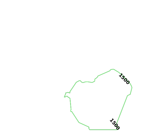
 The second group of isochrones is calculated using the following parameters:
The `solve_direction` is still `to_source` at this point, so
the second group of isochrones is calculated for leading **to**
DCA
* `source_node` is provided as a WKT point (`R_AIR`) paired with a
`NODE_WKTPOINT` [identifier](/content/graph_solver/network_graph_solver#identifiers)
* `max_solution_radius` is set for 1500 seconds' (or 25 minutes') worth of
travel surrounding the source node
* `num_levels` is set to `1` to only display one isochrone contour around
the source node
* `generate_image` is set to `True` to generate an image and output it to
the response
```python Request DCA Isochrone Image theme={null}
vis_isochrone_r_resp = kinetica.visualize_isochrone(
graph_name = GRAPH_DC,
source_node = R_AIR + " AS NODE_WKTPOINT",
max_solution_radius = 25 * 60,
num_levels = 1,
generate_image = True,
levels_table = TABLE_R_LVL,
style_options = OPTION_ISO_STYLE,
contour_options = OPTION_ISO_CONTOUR,
options = OPTION_ISO
)
```
The image is pulled from the response and written locally:
```python Write DCA Isochrone Image to Disk theme={null}
img = vis_isochrone_r_resp["image_data"]
img_isochrones_to_reagan = open(R_AIR_IMG, "wb")
img_isochrones_to_reagan.write(img)
img_isochrones_to_reagan.close()
```
The generated image for DCA isochrones:
The second group of isochrones is calculated using the following parameters:
The `solve_direction` is still `to_source` at this point, so
the second group of isochrones is calculated for leading **to**
DCA
* `source_node` is provided as a WKT point (`R_AIR`) paired with a
`NODE_WKTPOINT` [identifier](/content/graph_solver/network_graph_solver#identifiers)
* `max_solution_radius` is set for 1500 seconds' (or 25 minutes') worth of
travel surrounding the source node
* `num_levels` is set to `1` to only display one isochrone contour around
the source node
* `generate_image` is set to `True` to generate an image and output it to
the response
```python Request DCA Isochrone Image theme={null}
vis_isochrone_r_resp = kinetica.visualize_isochrone(
graph_name = GRAPH_DC,
source_node = R_AIR + " AS NODE_WKTPOINT",
max_solution_radius = 25 * 60,
num_levels = 1,
generate_image = True,
levels_table = TABLE_R_LVL,
style_options = OPTION_ISO_STYLE,
contour_options = OPTION_ISO_CONTOUR,
options = OPTION_ISO
)
```
The image is pulled from the response and written locally:
```python Write DCA Isochrone Image to Disk theme={null}
img = vis_isochrone_r_resp["image_data"]
img_isochrones_to_reagan = open(R_AIR_IMG, "wb")
img_isochrones_to_reagan.write(img)
img_isochrones_to_reagan.close()
```
The generated image for DCA isochrones:
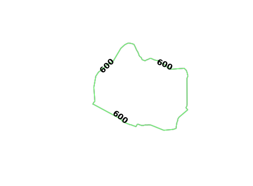
 Before the last example, the solve direction is updated to reflect that the
isochrones are calculated leading **from** Kinetica HQ:
```python Update Solve Orientation theme={null}
OPTION_ISO["solve_direction"] = "from_source"
```
Finally, the third group of isochrones can be calculated using the following
parameters:
* `source_node` is provided as a WKT point (`K_HQ`) paired with a
`NODE_WKTPOINT` [identifier](/content/graph_solver/network_graph_solver#identifiers)
* `max_solution_radius` is set for 600 seconds' (or 10 minutes') worth of
travel surrounding the source node
* `num_levels` is set to `1` to only display one isochrone contour around
the source node
* `generate_image` is set to `True` to generate an image and output it to
the response
```python Request Kinetica HQ Isochrone Image theme={null}
vis_isochrone_k1_resp = kinetica.visualize_isochrone(
graph_name = GRAPH_DC,
source_node = K_HQ + " AS NODE_WKTPOINT",
max_solution_radius = 10 * 60,
num_levels = 1,
generate_image = True,
levels_table = TABLE_K_LVL1,
style_options = OPTION_ISO_STYLE,
contour_options = OPTION_ISO_CONTOUR,
options = OPTION_ISO
)
```
The image is pulled from the response and written locally:
```python Write Kinetica HQ Isochrone Image to Disk theme={null}
img = vis_isochrone_k1_resp["image_data"]
img_isochrones_from_kinetica = open(K_HQ_IMG1, "wb")
img_isochrones_from_kinetica.write(img)
img_isochrones_from_kinetica.close()
```
The generated image for Kinetica HQ (leading **from**) isochrones:
Before the last example, the solve direction is updated to reflect that the
isochrones are calculated leading **from** Kinetica HQ:
```python Update Solve Orientation theme={null}
OPTION_ISO["solve_direction"] = "from_source"
```
Finally, the third group of isochrones can be calculated using the following
parameters:
* `source_node` is provided as a WKT point (`K_HQ`) paired with a
`NODE_WKTPOINT` [identifier](/content/graph_solver/network_graph_solver#identifiers)
* `max_solution_radius` is set for 600 seconds' (or 10 minutes') worth of
travel surrounding the source node
* `num_levels` is set to `1` to only display one isochrone contour around
the source node
* `generate_image` is set to `True` to generate an image and output it to
the response
```python Request Kinetica HQ Isochrone Image theme={null}
vis_isochrone_k1_resp = kinetica.visualize_isochrone(
graph_name = GRAPH_DC,
source_node = K_HQ + " AS NODE_WKTPOINT",
max_solution_radius = 10 * 60,
num_levels = 1,
generate_image = True,
levels_table = TABLE_K_LVL1,
style_options = OPTION_ISO_STYLE,
contour_options = OPTION_ISO_CONTOUR,
options = OPTION_ISO
)
```
The image is pulled from the response and written locally:
```python Write Kinetica HQ Isochrone Image to Disk theme={null}
img = vis_isochrone_k1_resp["image_data"]
img_isochrones_from_kinetica = open(K_HQ_IMG1, "wb")
img_isochrones_from_kinetica.write(img)
img_isochrones_from_kinetica.close()
```
The generated image for Kinetica HQ (leading **from**) isochrones:
 To find the shared area between the three contours that were just created,
the `ST_INTERSECTION()` geospatial function is used to join the three tables
together:
```python Geospatial Intersection via Join theme={null}
create_join_resp = kinetica.create_join_table(
join_table_name = TABLE_JOIN,
table_names = [
TABLE_D_LVL + " AS DULLES",
TABLE_K_LVL1 + " AS KINETICA",
TABLE_R_LVL + " AS REAGAN"
],
column_names = [
"ST_INTERSECTION(REAGAN.Isochrones, ST_INTERSECTION(KINETICA.Isochrones, DULLES.Isochrones)) AS shared_isochrones"
],
expressions = [],
options = {}
)
```
The shared area geometry output to WMS:
To find the shared area between the three contours that were just created,
the `ST_INTERSECTION()` geospatial function is used to join the three tables
together:
```python Geospatial Intersection via Join theme={null}
create_join_resp = kinetica.create_join_table(
join_table_name = TABLE_JOIN,
table_names = [
TABLE_D_LVL + " AS DULLES",
TABLE_K_LVL1 + " AS KINETICA",
TABLE_R_LVL + " AS REAGAN"
],
column_names = [
"ST_INTERSECTION(REAGAN.Isochrones, ST_INTERSECTION(KINETICA.Isochrones, DULLES.Isochrones)) AS shared_isochrones"
],
expressions = [],
options = {}
)
```
The shared area geometry output to WMS:
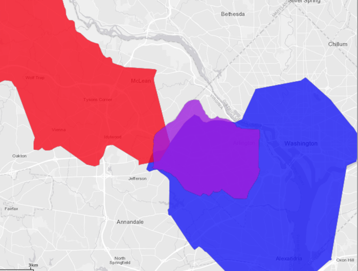
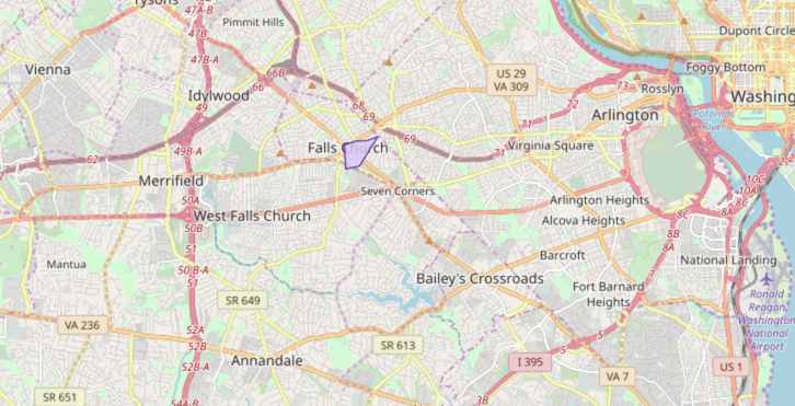 The three isochrones overlaid on top of each other:
* Red signifies being within 40 minutes of IAD
* Blue signifies being within 25 minutes of DCA
* Purple signifies being within 10 minutes of Kinetica HQ
The three isochrones overlaid on top of each other:
* Red signifies being within 40 minutes of IAD
* Blue signifies being within 25 minutes of DCA
* Purple signifies being within 10 minutes of Kinetica HQ
 ### Visualizing Isochrones Using WMS
To visualize isochrones via the `/wms` endpoint, the WMS
payload must be constructed. Consult [/wms](/content/api/rest/wms_rest) for more
information on WMS parameters, styles, and style options.
WMS payloads require a small set of standard parameters that will generally be
the same across all WMS requests:
```python Standard WMS Parameters theme={null}
"request": "GetMap",
"version": "1.1.1",
"format": "image/png",
```
The next settings inform WMS to generate isochrones (and to make Isochrones
parameters available for use) and to set the image width to `512` pixels. The
image height is set to `-1`, which the database will replace with the value
resulting from multiplying the aspect ratio by the image width.
```python Standard Isochrone Parameters theme={null}
"styles": "isochrone",
"image_width": 512,
"image_height": -1,
```
The following parameters define how the isochrones will be calculated. Notice
these are similar to the previous examples:
* `source_node` is provided as a WKT point (`K_HQ`) paired with a
`NODE_WKTPOINT` [identifier](/content/graph_solver/network_graph_solver#identifiers)
* `max_solution_radius` is set for 900 seconds' (or 15 minutes') worth of
travel surrounding the source node
* `num_levels` is set to `10` to 10 isochrone contours around
the source node
* `generate_image` is set to `True` to generate an image and output it to
the response
```python Kinetica HQ Isochrone Parameters theme={null}
"graph_name": GRAPH_DC,
"source_node": K_HQ + " AS NODE_WKTPOINT",
"max_solution_radius": "900",
"num_levels": "10",
"generate_image": "true",
"levels_table": TABLE_K_LVL2,
```
Isochrone style options are passed in using the constants:
```python Isochrone Style Parameters theme={null}
"line_size": OPTION_ISO_STYLE["line_size"],
"color": OPTION_ISO_STYLE["color"][2:], # remove the 0x
"bg_color": OPTION_ISO_STYLE["bg_color"][2:], # remove the 0x
"colormap": OPTION_ISO_STYLE["colormap"],
```
Isochrone contour options are passed in. Additional contour style parameters
are passed in for additional customization over the generated isochrones:
```python Isochrone Contour Parameters theme={null}
"projection": "plate_carree",
"search_radius": OPTION_ISO_CONTOUR["search_radius"],
"color_isolines": OPTION_ISO_CONTOUR["color_isolines"],
"add_labels": "false",
"gridding_method": OPTION_ISO_CONTOUR["gridding_method"],
"smoothing_factor": OPTION_ISO_CONTOUR["smoothing_factor"],
"max_search_cells": "100",
"min_grid_size": OPTION_ISO_CONTOUR["min_grid_size"],
"max_grid_size": OPTION_ISO_CONTOUR["max_grid_size"],
```
Lastly, isochrone options are passed in. Note the change in direction for the
`solve_direction` as we want isochrones leading **to** Kinetica HQ in this
instance.
```python Isochrone Solve & Output Parameters theme={null}
"solve_table": TABLE_K_ISO_SOLVE,
"is_replicated": OPTION_ISO["is_replicated"],
"concavity_level": OPTION_ISO["concavity_level"],
"solve_direction": "to_source"
```
The WMS request is sent and the image is pulled from the response and written
locally:
```python Request Isochrone Image theme={null}
params = urllib.urlencode(payload)
call_wms_request = requests.get(WMS_URL, auth=(username, password), params=params)
wms_img = call_wms_request.content
```
```python Write Isochrone Image to Disk theme={null}
img_isochrones_to_kinetica = open(K_HQ_IMG2, "wb")
img_isochrones_to_kinetica.write(wms_img)
img_isochrones_to_kinetica.close()
```
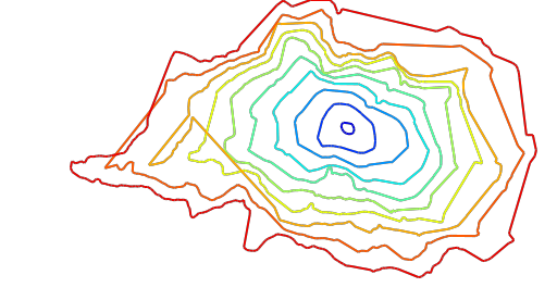
The generated image for Kinetica HQ (leading **to**) isochrones:
### Visualizing Isochrones Using WMS
To visualize isochrones via the `/wms` endpoint, the WMS
payload must be constructed. Consult [/wms](/content/api/rest/wms_rest) for more
information on WMS parameters, styles, and style options.
WMS payloads require a small set of standard parameters that will generally be
the same across all WMS requests:
```python Standard WMS Parameters theme={null}
"request": "GetMap",
"version": "1.1.1",
"format": "image/png",
```
The next settings inform WMS to generate isochrones (and to make Isochrones
parameters available for use) and to set the image width to `512` pixels. The
image height is set to `-1`, which the database will replace with the value
resulting from multiplying the aspect ratio by the image width.
```python Standard Isochrone Parameters theme={null}
"styles": "isochrone",
"image_width": 512,
"image_height": -1,
```
The following parameters define how the isochrones will be calculated. Notice
these are similar to the previous examples:
* `source_node` is provided as a WKT point (`K_HQ`) paired with a
`NODE_WKTPOINT` [identifier](/content/graph_solver/network_graph_solver#identifiers)
* `max_solution_radius` is set for 900 seconds' (or 15 minutes') worth of
travel surrounding the source node
* `num_levels` is set to `10` to 10 isochrone contours around
the source node
* `generate_image` is set to `True` to generate an image and output it to
the response
```python Kinetica HQ Isochrone Parameters theme={null}
"graph_name": GRAPH_DC,
"source_node": K_HQ + " AS NODE_WKTPOINT",
"max_solution_radius": "900",
"num_levels": "10",
"generate_image": "true",
"levels_table": TABLE_K_LVL2,
```
Isochrone style options are passed in using the constants:
```python Isochrone Style Parameters theme={null}
"line_size": OPTION_ISO_STYLE["line_size"],
"color": OPTION_ISO_STYLE["color"][2:], # remove the 0x
"bg_color": OPTION_ISO_STYLE["bg_color"][2:], # remove the 0x
"colormap": OPTION_ISO_STYLE["colormap"],
```
Isochrone contour options are passed in. Additional contour style parameters
are passed in for additional customization over the generated isochrones:
```python Isochrone Contour Parameters theme={null}
"projection": "plate_carree",
"search_radius": OPTION_ISO_CONTOUR["search_radius"],
"color_isolines": OPTION_ISO_CONTOUR["color_isolines"],
"add_labels": "false",
"gridding_method": OPTION_ISO_CONTOUR["gridding_method"],
"smoothing_factor": OPTION_ISO_CONTOUR["smoothing_factor"],
"max_search_cells": "100",
"min_grid_size": OPTION_ISO_CONTOUR["min_grid_size"],
"max_grid_size": OPTION_ISO_CONTOUR["max_grid_size"],
```
Lastly, isochrone options are passed in. Note the change in direction for the
`solve_direction` as we want isochrones leading **to** Kinetica HQ in this
instance.
```python Isochrone Solve & Output Parameters theme={null}
"solve_table": TABLE_K_ISO_SOLVE,
"is_replicated": OPTION_ISO["is_replicated"],
"concavity_level": OPTION_ISO["concavity_level"],
"solve_direction": "to_source"
```
The WMS request is sent and the image is pulled from the response and written
locally:
```python Request Isochrone Image theme={null}
params = urllib.urlencode(payload)
call_wms_request = requests.get(WMS_URL, auth=(username, password), params=params)
wms_img = call_wms_request.content
```
```python Write Isochrone Image to Disk theme={null}
img_isochrones_to_kinetica = open(K_HQ_IMG2, "wb")
img_isochrones_to_kinetica.write(wms_img)
img_isochrones_to_kinetica.close()
```
The generated image for Kinetica HQ (leading **to**) isochrones:
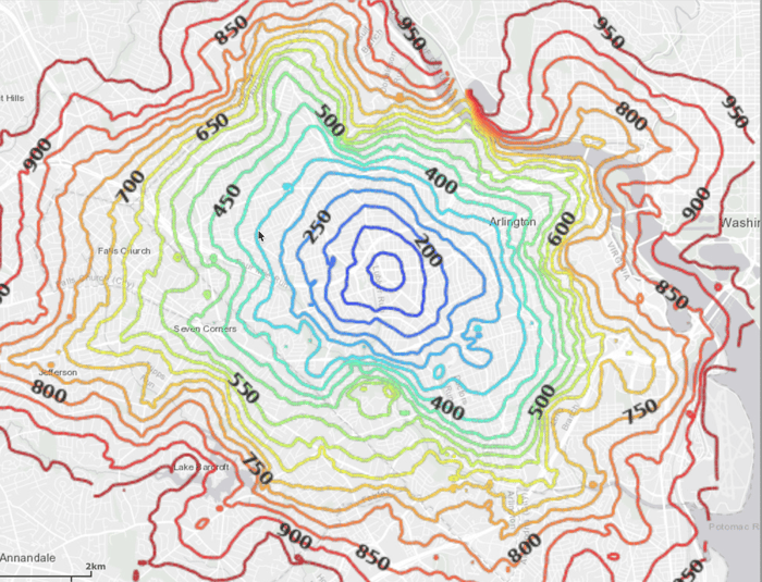
 With labels and map data underneath:
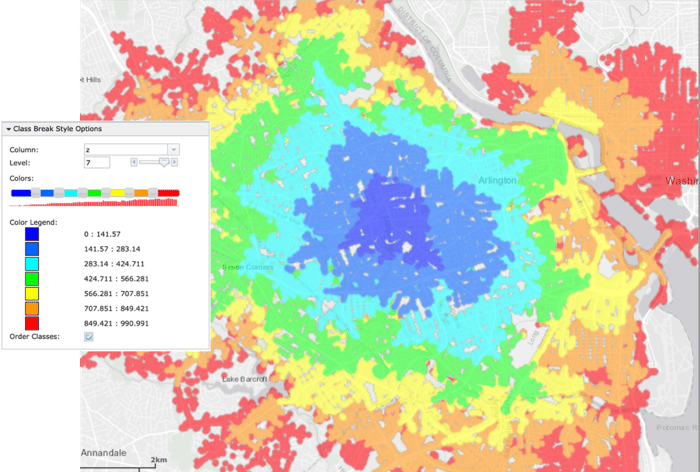
 Using the `solve_table` (`TABLE_K_ISO_SOLVE`), you can class break
on the `z` (cost) column in WMS to see individual points and their
relative cost:
Using the `solve_table` (`TABLE_K_ISO_SOLVE`), you can class break
on the `z` (cost) column in WMS to see individual points and their
relative cost:
 ## Download & Run
Included below is a complete example containing all the above requests, the data
files, and output.
* [Isochrones script](https://raw.githubusercontent.com/kineticadb/kinetica-docs/master/content/examples/python/isochrones.py)
* [DC shape data file](https://raw.githubusercontent.com/kineticadb/kinetica-docs/master/content/examples/data/dc_shape.csv)
* [Python output](https://raw.githubusercontent.com/kineticadb/kinetica-docs/master/content/examples/python/isochrones.out)
To run the complete sample, ensure that:
* the isochrones.py script is in the current directory
* the dc\_shape.csv file is in the current directory or use the
`data_dir` parameter to specify the local directory containing it
Then, run the following:
```bash title="Run Example" theme={null}
python isochrones.py [--url ] --username --password [--data_dir ]
```
## Download & Run
Included below is a complete example containing all the above requests, the data
files, and output.
* [Isochrones script](https://raw.githubusercontent.com/kineticadb/kinetica-docs/master/content/examples/python/isochrones.py)
* [DC shape data file](https://raw.githubusercontent.com/kineticadb/kinetica-docs/master/content/examples/data/dc_shape.csv)
* [Python output](https://raw.githubusercontent.com/kineticadb/kinetica-docs/master/content/examples/python/isochrones.out)
To run the complete sample, ensure that:
* the isochrones.py script is in the current directory
* the dc\_shape.csv file is in the current directory or use the
`data_dir` parameter to specify the local directory containing it
Then, run the following:
```bash title="Run Example" theme={null}
python isochrones.py [--url ] --username --password [--data_dir ]
```