> ## Documentation Index
> Fetch the complete documentation index at: https://docs.kinetica.com/llms.txt
> Use this file to discover all available pages before exploring further.
# Multiple Supply Demand in Python
> Supply chain optimization example in Python
The following is a complete example, using the *Python API*, of matching
stores (demands) to depots/trucks (suppliers) via the
[/match/graph](/content/api/rest/match_graph_rest) endpoint using an underlying graph
created from a modified OpenStreetMap (OSM) dataset. For more information on
Graphs & Solvers, see [Graphs & Solvers Concepts](/content/graph_solver/network_graph_solver).
## Prerequisites
The prerequisites for running the match graph example are listed below:
* Graph server enabled
* Python API
* [Match graph script](https://raw.githubusercontent.com/kineticadb/kinetica-docs/master/content/examples/python/graph/match_graph_dc_multi_supply_demand.py)
* [D.C. roads CSV file](https://raw.githubusercontent.com/kineticadb/kinetica-docs/master/content/examples/data/dc_roads.csv)
### Python API Installation
Depending on the target operating system, a Python virtual environment may need
to be installed first:
* [Python Virtual Environment](#python-virtual-environment)
The native *Kinetica Python API* is accessible through the following means:
* [PyPI](#pypi)
* [Git](#git)
#### Python Virtual Environment
A Python virtual environment is necessary to install in an operating environment
where Python is externally managed.
1. Install a Python virtual environment:
```bash theme={null}
python3 -m venv .venv
```
2. Activate the Python virtual environment:
```bash theme={null}
source .venv/bin/activate
```
#### PyPI
1. Install the API:
```bash theme={null}
pip3 install gpudb
```
2. Test the installation:
```python theme={null}
python3 -c "import gpudb;print('Import Successful')"
```
If *Import Successful* is displayed, the API has been installed as is ready
for use.
#### Git
1. In the desired directory, run the following, but be sure to replace
`` with the name of the installed Kinetica version,
e.g., `v7.2`:
```bash theme={null}
git clone -b release/ --single-branch https://github.com/kineticadb/kinetica-api-python.git
```
2. Change directory into the newly downloaded repository:
```bash theme={null}
cd kinetica-api-python
```
3. In the root directory of the unzipped repository, install the Kinetica API:
```bash theme={null}
sudo pip3 install .
```
4. Test the installation (*Python3* is necessary for running the API example):
```bash theme={null}
python3 examples/example.py
```
### Data File
The example script references the dc\_roads.csv data file,
mentioned in the [Prerequisites](#prerequisites), in the current local directory, by default.
This directory can specified as a parameter when running the script.
The `dc_shape` dataset is a HERE dataset and is analogous to most road network
datasets you could find in that it includes columns for the type of road, the
average speed, the direction of the road, a WKT linestring for its geographic
location, a unique ID integer for the road, and more. The graph used in the
example is created with two columns from the `dc_shape` dataset:
* `shape` -- a WKT linestring composed of points that make up various streets,
roads, highways, alleyways, and footpaths throughout Washington, D.C.
* `direction` -- an integer column that conveys information about the
directionality of the road, with forward meaning the direction in which
the way is drawn in OSM and backward being the opposite direction:
* `0` -- a forward one-way road
* `1` -- a two-way road
* `2` -- a backward one-way road
You'll notice later that the `shape` column is also part of an inline
calculation for distance as *weight* during graph creation using
the `ST_LENGTH` and `ST_NPOINTS`
[geospatial functions](/content/location_intelligence/geo_functions).
## Script Detail
This example is going to demonstrate matching supply trucks to different demand
points within Washington, D.C., relying on truck sizes, road weights, and
proximity to determine the best path between supply trucks and demands.
### Constants
Several constants are defined at the beginning of the script:
* `SCHEMA` -- the name of the schema in which the tables supporting the
graph creation and match operations will be created
The schema is created during the table setup portion of the
script because the schema must exist prior to creating the
tables that will later support the graph creation and match
operations.
* `TABLE_DC` -- the name of the table into which the D.C. roads dataset is
loaded
* `TABLE_D` / `TABLE_S` -- the names for the tables into which the datasets
in this file are loaded. `TABLE_D` is a record of each demand's (store) ID,
WKT location, size of demand, and their local supplier's ID; `TABLE_S` is
a record of each supplier's ID, WKT location, truck ID, and truck size.
* `GRAPH_DC` -- the D.C. roads graph
* `TABLE_GRAPH_DC_S1` / `TABLE_GRAPH_DC_S2` -- the names for the tables into
which the solutions are output
```python Constant Definitions theme={null}
SCHEMA = "graph_m_multi_supply_demand"
TABLE_DC = SCHEMA + ".dc_roads"
TABLE_D = SCHEMA + ".demands"
TABLE_S = SCHEMA + ".supplies"
GRAPH_DC = SCHEMA + ".dc_roads_graph"
TABLE_GRAPH_DC_S1 = GRAPH_DC + "_solved"
TABLE_GRAPH_DC_S2 = GRAPH_DC + "_solved_w_max_trip"
```
### Table Setup
Before the *supplies* and *demands* datasets are generated, the *D.C. roads*
dataset is loaded from a local CSV file. First, the *D.C. roads* table is
created using the [GPUdbTable](/content/api/python/source/gpudbtable)
interface:
```python Create D.C. Roads Table theme={null}
table_dc_obj = gpudb.GPUdbTable(
_type = [
["Feature_ID", "long"],
["osm_id", "string", "char16", "nullable"],
["code", "double", "nullable"],
["fclass", "string", "char32", "nullable"],
["name", "string", "char256", "nullable"],
["ref", "string", "char256", "nullable"],
["bidir", "string", "char2", "nullable"],
["maxspeed", "double", "nullable"],
["layer", "double", "nullable"],
["bridge", "string", "char2", "nullable"],
["tunnel", "string", "char2", "nullable"],
["WKT", "string", "wkt"],
["oneway", "int", "int8"],
["weight", "float"]
],
name = TABLE_DC,
db = kinetica,
options = {}
)
```
Then, the CSV file is uploaded into [KiFS](/content/tools/kifs) and loaded
into the table:
```python Populate D.C. Roads Table theme={null}
kinetica.create_directory("data", {"no_error_if_exists":"true"});
kinetica.upload_files("/data/" + CSV_FILE, open(csv_path, "rb").read())
kinetica.insert_records_from_files(TABLE_DC, ["kifs://data/" + CSV_FILE])
```
The *demands* table is also created using the
[GPUdbTable](/content/api/python/source/gpudbtable) interface:
```python Create Demands Table theme={null}
table_d_obj = gpudb.GPUdbTable(
_type = [
["store_id", "int", "int16"],
["store_location", "string", "wkt"],
["demand_size", "int", "int16"],
["supplier_id", "int", "int16"],
["priority", "int", "int16"]
],
name = TABLE_D,
db = kinetica,
options = {}
)
```
There should not be multiple demand records for the same supplier,
e.g., two separate demands of 5 and 10 for Store ID 1 should be
combined for one demand of 15
Then the *demands* records are defined and inserted into the table. Six
stores are created in various locations throughout the city with varying
demands but they all use the same supplier. Note that the higher the priority
number, the greater the priority (e.g., `3` is the highest priority in this
example and `0` is the lowest):
```python Populate Demands Table theme={null}
d_records = [
[11, "POINT(-77.0297975 38.896235)", 35, 1, 0],
[12, "POINT(-77.0286392 38.9169977)", 15, 1, 0],
[13, "POINT(-77.00128239999999 38.8748973)", 40, 1, 1],
[44, "POINT(-76.97952479999999 38.8995292)", 23, 1, 0],
[45, "POINT(-77.026516 38.9408711)", 28, 1, 2],
[46, "POINT(-77.0254317 38.8848442)", 25, 1, 3]
]
table_d_obj.insert_records(d_records)
```
Lastly, the *supplies* table is created using the
[GPUdbTable](/content/api/python/source/gpudbtable) interface:
```python Create Supplies Table theme={null}
table_s_obj = gpudb.GPUdbTable(
_type = [
["supplier_id", "int", "int16"],
["supplier_location", "string", "wkt"],
["truck_id", "int", "int16"],
["truck_size", "int", "int16"]
],
name = TABLE_S,
db = kinetica,
options = {}
)
```
Five *supplies* records are defined and inserted into the table: five trucks
with varying sizes are assigned to the same supplier.
```python Populate Supplies Table theme={null}
s_records = [
[1, "POINT(-77.0440586 38.9089819)", 21, 50],
[1, "POINT(-77.0440586 38.9089819)", 22, 50],
[1, "POINT(-77.0440586 38.9089819)", 23, 30],
[1, "POINT(-77.0440586 38.9089819)", 24, 20],
[1, "POINT(-77.0440586 38.9089819)", 25, 16]
]
table_s_obj.insert_records(s_records)
```
### Graph Creation
One graph is used for the match graph example utilized in the script:
`dc_roads_graph`, a graph based on the `dc_roads` dataset
(one of the CSV files mentioned in [Prerequisites](#prerequisites)).
The `dc_roads_graph` graph is created with the following
characteristics:
* It is [directed](/content/graph_solver/network_graph_solver#directed-graphs) because the roads in the graph
have directionality (one-way and two-way roads)
* It has no explicitly defined *nodes* because the example relies on implicit
*nodes* attached to the defined *edges*
* The *edges* are identified by `WKTLINE`, using WKT LINESTRINGs from the
`WKT` column of the `dc_roads` table. The road segments' directionality
(`DIRECTION`) is derived from the `oneway` column of the `dc_roads`
table.
* The *weights* (`VALUESPECIFIED`) are represented using the cost to travel
the segment found in the `weight` column of the `dc_roads` table. The
*weights* are matched to the *edges* using the same `WKT` column as *edges*
(`EDGE_WKTLINE`) and the same `oneway` column as the *edge* direction
(`EDGE_DIRECTION`).
* It has no inherent *restrictions* for any of the *nodes* or *edges* in the
graph
* It will be replaced with this instance of the graph if a graph of the same
name exists (`recreate`)
```python Create D.C. Road Network Graph theme={null}
create_dc_graph_response = kinetica.create_graph(
graph_name = GRAPH_DC,
directed_graph = True,
nodes = [],
edges = [
TABLE_DC + ".WKT AS WKTLINE",
TABLE_DC + ".oneway AS DIRECTION"
],
weights = [
TABLE_DC + ".WKT AS EDGE_WKTLINE",
TABLE_DC + ".oneway AS EDGE_DIRECTION",
TABLE_DC + ".weight AS VALUESPECIFIED"
],
restrictions = [],
options = {
"recreate": "true"
}
)
```
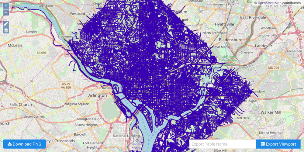
The graph output to WMS:
 ### Multiple Supply Demand with Priority
Both the *supplies* and *demands*
[match identifier combinations](/content/graph_solver/network_graph_solver#match-combinations) are provided to the
[/match/graph](/content/api/rest/match_graph_rest) endpoint so the graph
server can match the supply trucks to the demand locations and with respect
to priority. Using the multiple supply demand match solver results in a solution
table for each unique supplier ID; in this case, one table is created:
`dc_roads_graph_solved`.
```python Match Graph to Supply & Demand with Priority theme={null}
match_graph_dc_resp = kinetica.match_graph(
graph_name = GRAPH_DC,
sample_points = [
TABLE_D + ".store_id AS DEMAND_ID",
TABLE_D + ".store_location AS DEMAND_WKTPOINT",
TABLE_D + ".demand_size AS DEMAND_SIZE",
TABLE_D + ".supplier_id AS DEMAND_REGION_ID",
TABLE_D + ".priority AS PRIORITY",
"",
TABLE_S + ".supplier_id AS SUPPLY_REGION_ID",
TABLE_S + ".supplier_location AS SUPPLY_WKTPOINT",
TABLE_S + ".truck_id AS SUPPLY_ID",
TABLE_S + ".truck_size AS SUPPLY_SIZE"
],
solve_method = "match_supply_demand",
solution_table = TABLE_GRAPH_DC_S1,
options = {}
)
```
The example script utilizes [/get/records](/content/api/rest/get_records_rest)
to extract the results from the solution table:
```text Match Graph to Supply & Demand with Priority Solution theme={null}
+------------+-------------+------------------------+----------+
| Truck ID | Store IDs | Store Drops | Cost |
|------------+-------------+------------------------+----------|
| 24 | (46) | (20.000) | 0.409533 |
| 25 | (46,11) | (5.000,11.000) | 0.412311 |
| 21 | (13,11) | (40.000,10.000) | 0.741923 |
| 23 | (45,12) | (28.000,2.000) | 1.0872 |
| 22 | (12,44,11) | (13.000,23.000,14.000) | 1.28554 |
+------------+-------------+------------------------+----------+
```
The WKT route was left out of the displayed results for
readability.
### Solution Analysis
For each truck from the *supplies* table that is involved in the solution, the
solution table presents the store(s) visited (by ID), how much "supply" is
dropped off at each store, the route taken to the store(s) and back to the
supplier, and the cost for the entire route.
Based on the results, you can see that the priority stores' demands were met
first: store IDs 46, 45, and 13. Truck ID 24 made a stop at Store 46 and dropped
off its entire supply. Once a truck has exhausted its supply in the solution, it
is no longer used. Truck ID 25 made a stop at Store ID 46 and 11: it stopped at
Store 46 to fulfill the rest of the store's demand and supplied Store 11 with
the rest of its available supply. Trucks will drop off as much
supply as they are able; if some supply is left on the truck after a drop-off,
the truck will continue to the next most optimal drop-off location regardless
of priority. Truck ID 23 made a stop at Store ID 45 to fulfill the store's
entire demand and Store ID 12 to drop off the rest of its available supply.
Truck ID 21 made a stop at Store ID 13 to fulfill the store's entire demand
and Store ID 11 to drop off the rest of its available supply. Truck ID 22
made a stop at Store ID 12, 44, and 11 to either fulfill the store's entire
demand (44) or to complete the rest of the store's demand (12, 11).
### Multiple Supply Demand with Priority and Max Trip Cost
Similarly to the example above, both the *supplies* and *demands*
[match identifier combinations](/content/graph_solver/network_graph_solver#match-combinations) are provided to the
[/match/graph](/content/api/rest/match_graph_rest) endpoint so the graph
server can match the supply trucks to the demand locations and with respect
to priority and the max trip cost. Max trip cost affects this example by
preventing trucks from supplying another store if the cost to travel to
that store is greater than the provided cost. Using the multiple supply demand
match solver results in a solution table for each unique supplier ID; in this
case, one table is created: `dc_roads_graph_solved_w_max_trip`.
```python Match Graph to Supply & Demand with Priority & Max Trip Cost theme={null}
match_graph_dc_resp = kinetica.match_graph(
graph_name = GRAPH_DC,
sample_points = [
TABLE_D + ".store_id AS DEMAND_ID",
TABLE_D + ".store_location AS DEMAND_WKTPOINT",
TABLE_D + ".demand_size AS DEMAND_SIZE",
TABLE_D + ".supplier_id AS DEMAND_REGION_ID",
TABLE_D + ".priority AS PRIORITY",
"",
TABLE_S + ".supplier_id AS SUPPLY_REGION_ID",
TABLE_S + ".supplier_location AS SUPPLY_WKTPOINT",
TABLE_S + ".truck_id AS SUPPLY_ID",
TABLE_S + ".truck_size AS SUPPLY_SIZE"
],
solve_method = "match_supply_demand",
solution_table = TABLE_GRAPH_DC_S2,
options = {
"max_trip_cost": "0.6",
"aggregated_output": "true"
}
)
```
The example script utilizes [/get/records](/content/api/rest/get_records_rest)
again to extract the results from the second solution table:
```text Match Graph to Supply & Demand with Priority & Max Trip Cost Solution theme={null}
+------------+-------------+------------------------+----------+
| Truck ID | Store IDs | Store Drops | Cost |
|------------+-------------+------------------------+----------|
| 24 | (46) | (20.000) | 0.409533 |
| 25 | (46,11) | (5.000,11.000) | 0.412311 |
| 21 | (13,11) | (40.000,10.000) | 0.741923 |
| 23 | (45,12) | (28.000,2.000) | 1.0872 |
| 22 | (12,44,11) | (13.000,23.000,14.000) | 1.28554 |
+------------+-------------+------------------------+----------+
```
The WKT route was left out of the displayed results for
readability.
## Download & Run
Included below is a complete example containing all the above requests, the data
files, and output.
* [Match graph script](https://raw.githubusercontent.com/kineticadb/kinetica-docs/master/content/examples/python/graph/match_graph_dc_multi_supply_demand.py)
* [D.C. roads data file](https://raw.githubusercontent.com/kineticadb/kinetica-docs/master/content/examples/data/dc_roads.csv)
* [Python output](https://raw.githubusercontent.com/kineticadb/kinetica-docs/master/content/examples/python/graph/match_graph_dc_multi_supply_demand.out)
To run the complete sample, ensure that:
* the match\_graph\_dc\_multi\_supply\_demand.py script is in the
current directory
* the dc\_roads.csv file is in the current directory or use the
`data_dir` parameter to specify the local directory containing it
Then, run the following:
```bash title="Run Example" theme={null}
python match_graph_dc_multi_supply_demand.py [--url ] --username --password [--data_dir ]
```
### Multiple Supply Demand with Priority
Both the *supplies* and *demands*
[match identifier combinations](/content/graph_solver/network_graph_solver#match-combinations) are provided to the
[/match/graph](/content/api/rest/match_graph_rest) endpoint so the graph
server can match the supply trucks to the demand locations and with respect
to priority. Using the multiple supply demand match solver results in a solution
table for each unique supplier ID; in this case, one table is created:
`dc_roads_graph_solved`.
```python Match Graph to Supply & Demand with Priority theme={null}
match_graph_dc_resp = kinetica.match_graph(
graph_name = GRAPH_DC,
sample_points = [
TABLE_D + ".store_id AS DEMAND_ID",
TABLE_D + ".store_location AS DEMAND_WKTPOINT",
TABLE_D + ".demand_size AS DEMAND_SIZE",
TABLE_D + ".supplier_id AS DEMAND_REGION_ID",
TABLE_D + ".priority AS PRIORITY",
"",
TABLE_S + ".supplier_id AS SUPPLY_REGION_ID",
TABLE_S + ".supplier_location AS SUPPLY_WKTPOINT",
TABLE_S + ".truck_id AS SUPPLY_ID",
TABLE_S + ".truck_size AS SUPPLY_SIZE"
],
solve_method = "match_supply_demand",
solution_table = TABLE_GRAPH_DC_S1,
options = {}
)
```
The example script utilizes [/get/records](/content/api/rest/get_records_rest)
to extract the results from the solution table:
```text Match Graph to Supply & Demand with Priority Solution theme={null}
+------------+-------------+------------------------+----------+
| Truck ID | Store IDs | Store Drops | Cost |
|------------+-------------+------------------------+----------|
| 24 | (46) | (20.000) | 0.409533 |
| 25 | (46,11) | (5.000,11.000) | 0.412311 |
| 21 | (13,11) | (40.000,10.000) | 0.741923 |
| 23 | (45,12) | (28.000,2.000) | 1.0872 |
| 22 | (12,44,11) | (13.000,23.000,14.000) | 1.28554 |
+------------+-------------+------------------------+----------+
```
The WKT route was left out of the displayed results for
readability.
### Solution Analysis
For each truck from the *supplies* table that is involved in the solution, the
solution table presents the store(s) visited (by ID), how much "supply" is
dropped off at each store, the route taken to the store(s) and back to the
supplier, and the cost for the entire route.
Based on the results, you can see that the priority stores' demands were met
first: store IDs 46, 45, and 13. Truck ID 24 made a stop at Store 46 and dropped
off its entire supply. Once a truck has exhausted its supply in the solution, it
is no longer used. Truck ID 25 made a stop at Store ID 46 and 11: it stopped at
Store 46 to fulfill the rest of the store's demand and supplied Store 11 with
the rest of its available supply. Trucks will drop off as much
supply as they are able; if some supply is left on the truck after a drop-off,
the truck will continue to the next most optimal drop-off location regardless
of priority. Truck ID 23 made a stop at Store ID 45 to fulfill the store's
entire demand and Store ID 12 to drop off the rest of its available supply.
Truck ID 21 made a stop at Store ID 13 to fulfill the store's entire demand
and Store ID 11 to drop off the rest of its available supply. Truck ID 22
made a stop at Store ID 12, 44, and 11 to either fulfill the store's entire
demand (44) or to complete the rest of the store's demand (12, 11).
### Multiple Supply Demand with Priority and Max Trip Cost
Similarly to the example above, both the *supplies* and *demands*
[match identifier combinations](/content/graph_solver/network_graph_solver#match-combinations) are provided to the
[/match/graph](/content/api/rest/match_graph_rest) endpoint so the graph
server can match the supply trucks to the demand locations and with respect
to priority and the max trip cost. Max trip cost affects this example by
preventing trucks from supplying another store if the cost to travel to
that store is greater than the provided cost. Using the multiple supply demand
match solver results in a solution table for each unique supplier ID; in this
case, one table is created: `dc_roads_graph_solved_w_max_trip`.
```python Match Graph to Supply & Demand with Priority & Max Trip Cost theme={null}
match_graph_dc_resp = kinetica.match_graph(
graph_name = GRAPH_DC,
sample_points = [
TABLE_D + ".store_id AS DEMAND_ID",
TABLE_D + ".store_location AS DEMAND_WKTPOINT",
TABLE_D + ".demand_size AS DEMAND_SIZE",
TABLE_D + ".supplier_id AS DEMAND_REGION_ID",
TABLE_D + ".priority AS PRIORITY",
"",
TABLE_S + ".supplier_id AS SUPPLY_REGION_ID",
TABLE_S + ".supplier_location AS SUPPLY_WKTPOINT",
TABLE_S + ".truck_id AS SUPPLY_ID",
TABLE_S + ".truck_size AS SUPPLY_SIZE"
],
solve_method = "match_supply_demand",
solution_table = TABLE_GRAPH_DC_S2,
options = {
"max_trip_cost": "0.6",
"aggregated_output": "true"
}
)
```
The example script utilizes [/get/records](/content/api/rest/get_records_rest)
again to extract the results from the second solution table:
```text Match Graph to Supply & Demand with Priority & Max Trip Cost Solution theme={null}
+------------+-------------+------------------------+----------+
| Truck ID | Store IDs | Store Drops | Cost |
|------------+-------------+------------------------+----------|
| 24 | (46) | (20.000) | 0.409533 |
| 25 | (46,11) | (5.000,11.000) | 0.412311 |
| 21 | (13,11) | (40.000,10.000) | 0.741923 |
| 23 | (45,12) | (28.000,2.000) | 1.0872 |
| 22 | (12,44,11) | (13.000,23.000,14.000) | 1.28554 |
+------------+-------------+------------------------+----------+
```
The WKT route was left out of the displayed results for
readability.
## Download & Run
Included below is a complete example containing all the above requests, the data
files, and output.
* [Match graph script](https://raw.githubusercontent.com/kineticadb/kinetica-docs/master/content/examples/python/graph/match_graph_dc_multi_supply_demand.py)
* [D.C. roads data file](https://raw.githubusercontent.com/kineticadb/kinetica-docs/master/content/examples/data/dc_roads.csv)
* [Python output](https://raw.githubusercontent.com/kineticadb/kinetica-docs/master/content/examples/python/graph/match_graph_dc_multi_supply_demand.out)
To run the complete sample, ensure that:
* the match\_graph\_dc\_multi\_supply\_demand.py script is in the
current directory
* the dc\_roads.csv file is in the current directory or use the
`data_dir` parameter to specify the local directory containing it
Then, run the following:
```bash title="Run Example" theme={null}
python match_graph_dc_multi_supply_demand.py [--url ] --username --password [--data_dir ]
```