> ## Documentation Index
> Fetch the complete documentation index at: https://docs.kinetica.com/llms.txt
> Use this file to discover all available pages before exploring further.
# Map Matching with Python
> An end-to-end example of map matching in the Python API
The following is a complete example, using the *Python API*, of matching
GPS sample data to road network data via the
[/match/graph](/content/api/rest/match_graph_rest) endpoint. For more information on
Graphs & Solvers, see [Graphs & Solvers Concepts](/content/graph_solver/network_graph_solver).
## Prerequisites
The prerequisites for running the match graph example are listed below:
* Graph server enabled
* Python API
* [Match graph script](https://raw.githubusercontent.com/kineticadb/kinetica-docs/master/content/examples/python/graph/match_graph_seattle_markov.py)
* Two CSV files:
* [Seattle road network](https://raw.githubusercontent.com/kineticadb/kinetica-docs/master/content/examples/data/road_weights.csv)
* [Raw GPS samples](https://raw.githubusercontent.com/kineticadb/kinetica-docs/master/content/examples/data/mm_raw_gps.csv)
### Python API Installation
Depending on the target operating system, a Python virtual environment may need
to be installed first:
* [Python Virtual Environment](#python-virtual-environment)
The native *Kinetica Python API* is accessible through the following means:
* [PyPI](#pypi)
* [Git](#git)
#### Python Virtual Environment
A Python virtual environment is necessary to install in an operating environment
where Python is externally managed.
1. Install a Python virtual environment:
```bash theme={null}
python3 -m venv .venv
```
2. Activate the Python virtual environment:
```bash theme={null}
source .venv/bin/activate
```
#### PyPI
1. Install the API:
```bash theme={null}
pip3 install gpudb
```
2. Test the installation:
```python theme={null}
python3 -c "import gpudb;print('Import Successful')"
```
If *Import Successful* is displayed, the API has been installed as is ready
for use.
#### Git
1. In the desired directory, run the following, but be sure to replace
`` with the name of the installed Kinetica version,
e.g., `v7.2`:
```bash theme={null}
git clone -b release/ --single-branch https://github.com/kineticadb/kinetica-api-python.git
```
2. Change directory into the newly downloaded repository:
```bash theme={null}
cd kinetica-api-python
```
3. In the root directory of the unzipped repository, install the Kinetica API:
```bash theme={null}
sudo pip3 install .
```
4. Test the installation (*Python3* is necessary for running the API example):
```bash theme={null}
python3 examples/example.py
```
### Data Files
The example script references two data files, as mentioned in the
[Prerequisites](#prerequisites), in the current local directory, by default. This directory
can specified as a parameter when running the script.
## Script Detail
This example is going to demonstrate matching raw GPS points to a Seattle road
network, relying on timestamps to determine the start and end point of the GPS
signal.
### Constants
Several constants are defined at the beginning of the script:
* `SCHEMA` -- the name of the schema in which the tables supporting the
graph creation and match operations will be created
The schema is created during the table setup portion of the
script because the schema must exist prior to creating the
tables that will later support the graph creation and match
operations.
* `TABLE_SRN` -- the name of the table into which the Seattle road network
dataset is loaded
* `TABLE_GPS` -- the name of the table into which the raw GPS samples dataset
is loaded
* `TABLE_SOLUTION1` / `TABLE_SOLUTION2` -- the names of the tables into
which the solutions are output
* `GRAPH_S` -- the Seattle road network graph
```python Constant Definitions theme={null}
SCHEMA = "graph_m_seattle_markov"
TABLE_SRN = SCHEMA + ".seattle_road_network"
TABLE_GPS = SCHEMA + ".raw_gps_samples"
TABLE_SOLUTION1 = TABLE_SRN + "_match_solved"
TABLE_SOLUTION2 = TABLE_SOLUTION1 + "_w_filter_folding"
GRAPH_S = SCHEMA + ".seattle_road_network_graph"
```
### Graph Creation
One graph is used for the match graph example utilized in the script:
`seattle_road_network_graph`, a graph based on the `road_weights` dataset
(one of the CSV files mentioned in [Prerequisites](#prerequisites)).
The `seattle_road_network_graph` graph is created with the following
characteristics:
* It is [directed](/content/graph_solver/network_graph_solver#directed-graphs) because the roads in the graph have
directionality (one-way and two-way roads)
* It has no explicitly defined *nodes* because the example relies on implicit
*nodes* attached to the defined *edges*
* The *edges* are identified by `WKTLINE`, using WKT LINESTRINGs from the
`WKTLINE` column of the `seattle_road_network` table. The road segments'
directionality (`DIRECTION`) is derived from the `TwoWay` column of the
`seattle_road_network` table.
* The *weights* (`VALUESPECIFIED`) are represented using the time taken to
travel the segment found in the `time` column of the
`seattle_road_network` table. The *weights* are matched to the *edges* using
the same `WKTLINE` column as *edges* (`EDGE_WKTLINE`) and the same
`TwoWay` column as the *edge* direction (`EDGE_DIRECTION`).
* It has no inherent *restrictions* for any of the *nodes* or *edges* in the
graph
* It will be replaced with this instance of the graph if a graph of the same
name exists (`recreate`)
```python Create Seattle Road Network Graph theme={null}
create_s_graph_response = kdb.create_graph(
graph_name = GRAPH_S,
directed_graph = True,
nodes = [],
edges = [
TABLE_SRN + ".WKTLINE AS WKTLINE",
TABLE_SRN + ".TwoWay AS DIRECTION"
],
weights = [
TABLE_SRN + ".WKTLINE AS EDGE_WKTLINE",
TABLE_SRN + ".TwoWay AS EDGE_DIRECTION",
TABLE_SRN + ".time AS VALUESPECIFIED"
],
restrictions = [],
options = {
"recreate": "true"
}
)
```
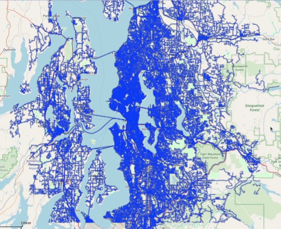
The graph output to WMS:
 ### Matching the Graph without Fold-over Filtering
Matching to a graph typically requires another table's worth of data. In this
case, the data that will be matched to the graph will come from the
`mm_raw_gps` dataset (the other CSV file mentioned in [Prerequisites](#prerequisites)). The
sample points are defined using the `lon` and `lat` columns as the X and Y
coordinates for each sample point; the `datetime` column is used for each
sample point's timestamp. The time component is required for determining the
start and end points of the samples.
```python Match Graph to GPS Data without Fold-over Filtering theme={null}
match_s_graph_response = kdb.match_graph(
graph_name = GRAPH_S,
sample_points = [
TABLE_GPS + ".lon AS X",
TABLE_GPS + ".lat AS Y",
TABLE_GPS + ".datetime AS TIME"
],
solve_method = "markov_chain",
solution_table = TABLE_SOLUTION1,
options = {}
)
```
The mean square error score is returned:
```text Match Graph to GPS Data without Fold-over Filtering Score theme={null}
Score for how well the samples matched to the graph (closer to 0 is better): 0.000036783752876
```
The solution output to WMS:
### Matching the Graph without Fold-over Filtering
Matching to a graph typically requires another table's worth of data. In this
case, the data that will be matched to the graph will come from the
`mm_raw_gps` dataset (the other CSV file mentioned in [Prerequisites](#prerequisites)). The
sample points are defined using the `lon` and `lat` columns as the X and Y
coordinates for each sample point; the `datetime` column is used for each
sample point's timestamp. The time component is required for determining the
start and end points of the samples.
```python Match Graph to GPS Data without Fold-over Filtering theme={null}
match_s_graph_response = kdb.match_graph(
graph_name = GRAPH_S,
sample_points = [
TABLE_GPS + ".lon AS X",
TABLE_GPS + ".lat AS Y",
TABLE_GPS + ".datetime AS TIME"
],
solve_method = "markov_chain",
solution_table = TABLE_SOLUTION1,
options = {}
)
```
The mean square error score is returned:
```text Match Graph to GPS Data without Fold-over Filtering Score theme={null}
Score for how well the samples matched to the graph (closer to 0 is better): 0.000036783752876
```
The solution output to WMS:
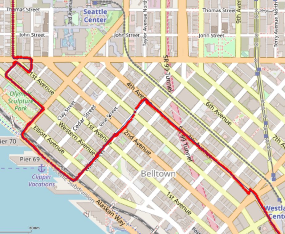
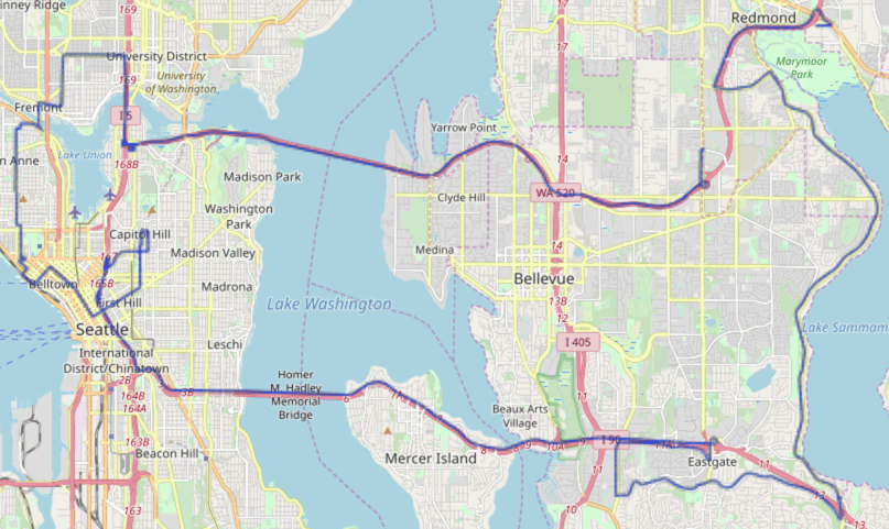 To demonstrate how successful the map matching solution was, the raw GPS
samples can be overlaid on top of the solution using WMS. Below is a sample
of the total solution.
To demonstrate how successful the map matching solution was, the raw GPS
samples can be overlaid on top of the solution using WMS. Below is a sample
of the total solution.
 ### Matching the Graph with Fold-over Filtering
To demonstrate how removing fold-over paths from the match solution yields
a different but more accurate score, a similar [/match/graph](/content/api/rest/match_graph_rest)
request to the above can be made but note that removing fold-over paths, e.g.,
setting `filter_folding_paths` to `true`, can increase execution time.
```python Match Graph to GPS Data with Fold-over Filtering theme={null}
match_s_graph_response = kdb.match_graph(
graph_name = GRAPH_S,
sample_points = [
TABLE_GPS + ".lon AS X",
TABLE_GPS + ".lat AS Y",
TABLE_GPS + ".datetime AS TIME"
],
solve_method = "markov_chain",
solution_table = TABLE_SOLUTION2,
options = {
"filter_folding_paths": "true"
}
)
```
The mean square error score is returned:
```text Match Graph to GPS Data with Fold-over Filtering Score theme={null}
Score for how well the samples matched to the graph with filter folding (closer to 0 is better): 0.000037545614759
```
## Download & Run
Included below is a complete example containing all the above requests, the data
files, and output.
* [Match graph script](https://raw.githubusercontent.com/kineticadb/kinetica-docs/master/content/examples/python/graph/match_graph_seattle_markov.py)
* [Seattle road network data file](https://raw.githubusercontent.com/kineticadb/kinetica-docs/master/content/examples/data/road_weights.csv)
* [Raw GPS samples data file](https://raw.githubusercontent.com/kineticadb/kinetica-docs/master/content/examples/data/mm_raw_gps.csv)
* [Python output](https://raw.githubusercontent.com/kineticadb/kinetica-docs/master/content/examples/python/graph/match_graph_seattle_markov.out)
To run the complete sample, ensure that:
* the match\_graph\_seattle\_markov.py script is in the current
directory
* the road\_weights.csv & mm\_raw\_gps.csv files are
in the current directory or use the `data_dir` parameter to specify the
local directory containing it
Then, run the following:
```bash title="Run Example" theme={null}
python match_graph_seattle_markov.py [--url ] --username --password [--data_dir ]
```
### Matching the Graph with Fold-over Filtering
To demonstrate how removing fold-over paths from the match solution yields
a different but more accurate score, a similar [/match/graph](/content/api/rest/match_graph_rest)
request to the above can be made but note that removing fold-over paths, e.g.,
setting `filter_folding_paths` to `true`, can increase execution time.
```python Match Graph to GPS Data with Fold-over Filtering theme={null}
match_s_graph_response = kdb.match_graph(
graph_name = GRAPH_S,
sample_points = [
TABLE_GPS + ".lon AS X",
TABLE_GPS + ".lat AS Y",
TABLE_GPS + ".datetime AS TIME"
],
solve_method = "markov_chain",
solution_table = TABLE_SOLUTION2,
options = {
"filter_folding_paths": "true"
}
)
```
The mean square error score is returned:
```text Match Graph to GPS Data with Fold-over Filtering Score theme={null}
Score for how well the samples matched to the graph with filter folding (closer to 0 is better): 0.000037545614759
```
## Download & Run
Included below is a complete example containing all the above requests, the data
files, and output.
* [Match graph script](https://raw.githubusercontent.com/kineticadb/kinetica-docs/master/content/examples/python/graph/match_graph_seattle_markov.py)
* [Seattle road network data file](https://raw.githubusercontent.com/kineticadb/kinetica-docs/master/content/examples/data/road_weights.csv)
* [Raw GPS samples data file](https://raw.githubusercontent.com/kineticadb/kinetica-docs/master/content/examples/data/mm_raw_gps.csv)
* [Python output](https://raw.githubusercontent.com/kineticadb/kinetica-docs/master/content/examples/python/graph/match_graph_seattle_markov.out)
To run the complete sample, ensure that:
* the match\_graph\_seattle\_markov.py script is in the current
directory
* the road\_weights.csv & mm\_raw\_gps.csv files are
in the current directory or use the `data_dir` parameter to specify the
local directory containing it
Then, run the following:
```bash title="Run Example" theme={null}
python match_graph_seattle_markov.py [--url ] --username --password [--data_dir ]
```