> ## Documentation Index
> Fetch the complete documentation index at: https://docs.kinetica.com/llms.txt
> Use this file to discover all available pages before exploring further.
# Querying Social Graphs in Python
> An example of querying a social graph with Kinetica (no external dataset required)
export const VideoEmbed = ({id, thumb, title, caption, maxWidth}) => {
const [playing, setPlaying] = useState(false);
const [hover, setHover] = useState(false);
const label = title ? `Play video: ${title}` : "Play video";
return
{playing ? : }
{(title || caption) &&
{title &&
{title}
}
{caption &&
{caption}
}
}
;
};
The following is a complete example, using the *Python API*, of querying social
relationship data via the [/query/graph](/content/api/rest/query_graph_rest) endpoint. For
more information on Graphs & Solvers, see
[Graphs & Solvers Concepts](/content/graph_solver/network_graph_solver).
## Prerequisites
The prerequisites for running the query graph example are listed below:
* Graph server enabled
* Python API
* [Query graph script](https://raw.githubusercontent.com/kineticadb/kinetica-docs/master/content/examples/python/graph/query_graph_social.py)
### Python API Installation
Depending on the target operating system, a Python virtual environment may need
to be installed first:
* [Python Virtual Environment](#python-virtual-environment)
The native *Kinetica Python API* is accessible through the following means:
* [PyPI](#pypi)
* [Git](#git)
#### Python Virtual Environment
A Python virtual environment is necessary to install in an operating environment
where Python is externally managed.
1. Install a Python virtual environment:
```bash theme={null}
python3 -m venv .venv
```
2. Activate the Python virtual environment:
```bash theme={null}
source .venv/bin/activate
```
#### PyPI
1. Install the API:
```bash theme={null}
pip3 install gpudb
```
2. Test the installation:
```python theme={null}
python3 -c "import gpudb;print('Import Successful')"
```
If *Import Successful* is displayed, the API has been installed as is ready
for use.
#### Git
1. In the desired directory, run the following, but be sure to replace
`` with the name of the installed Kinetica version,
e.g., `v7.2`:
```bash theme={null}
git clone -b release/ --single-branch https://github.com/kineticadb/kinetica-api-python.git
```
2. Change directory into the newly downloaded repository:
```bash theme={null}
cd kinetica-api-python
```
3. In the root directory of the unzipped repository, install the Kinetica API:
```bash theme={null}
sudo pip3 install .
```
4. Test the installation (*Python3* is necessary for running the API example):
```bash theme={null}
python3 examples/example.py
```
## Script Detail
This example is going to demonstrate querying a social network of relationships
between friends and family for:
* people directly or indirectly known to a given person who are interested in
chess but not known through family
* people directly known to a given gender
* people who are of a given gender or interested in chess
* people directly or indirectly known to a given gender who are interested in
chess
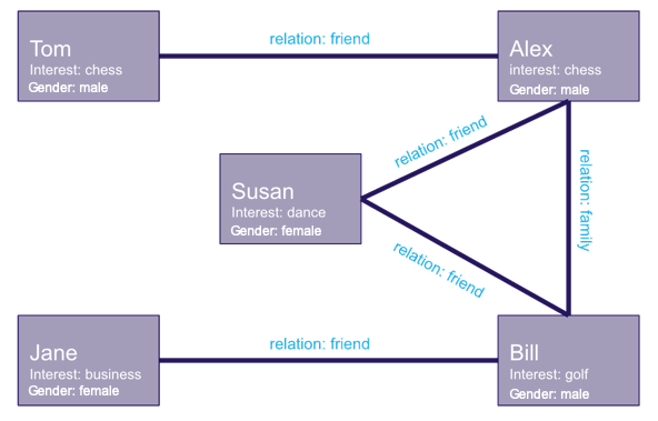
The graph queried in the examples below looks like this:
### Constants
Several constants are defined at the beginning of the script:
* `DEFAULT_SCHEMA` -- the name of the schema in which the tables supporting
the graph creation and match operations will be created, if one is not
specified on the command line
The schema is created during the table setup portion of the
script (if it doesn't already exist) because the schema must
exist prior to creating the tables that will later support the
graph creation and match operations.
* `people_table` / `knows_table` -- the names for the tables into which the
datasets generated in this file are loaded. These datasets will serve as the
basis for the social relationships graph. `people_table` is a record of a
person's name, age, and interest; `knows_table` defines the relationships
between the people
* `social_graph` -- the social relationships graph
* `TABLE_Q1` / `TABLE_Q2` / `TABLE_Q3` / `TABLE_Q4` -- the resulting
adjacency (edge) tables from the four query examples performed in the script
* `TABLE_Q1_TARGETS` / `TABLE_Q2_TARGETS` / `TABLE_Q3_TARGETS` /
`TABLE_Q4_TARGETS`-- the target (node) tables from the four examples
```python Constant Definitions theme={null}
DEFAULT_SCHEMA = "graph_q_social"
people_table = 'people'
knows_table = 'knows'
social_graph = 'social_relationships'
TABLE_Q1 = social_graph + "_queried_jane_to_chess"
TABLE_Q1_TARGETS = TABLE_Q1 + "_nodes"
TABLE_Q2 = social_graph + "_queried_males"
TABLE_Q2_TARGETS = TABLE_Q2 + "_nodes"
TABLE_Q3 = social_graph + "_queried_females_or_chess"
TABLE_Q3_TARGETS = TABLE_Q3 + "_nodes"
TABLE_Q4 = social_graph + "_queried_females_to_chess"
TABLE_Q4_TARGETS = TABLE_Q4 + "_nodes"
```
### Table Setup
As mentioned previously, there are two tables used in the graph creation step.
The first of these tables is the *people* table. It is created using the
[GPUdbTable](/content/api/python/source/gpudbtable) interface:
```python Create People Table theme={null}
table_p_obj = gpudb.GPUdbTable(
_type = [
["name", "string", "char16"],
["age", "int"],
["interest", "string", "char16"],
["gender", "string", "char8"]
],
name = people_table,
db = kinetica,
options = {}
)
```
Finally, the *people* records are defined and inserted:
```python Populate People Table theme={null}
p_records = [
["Susan", 22, "dance", "female"],
["Bill", 60, "golf", "male"],
["Alex", 34, "chess", "male"],
["Jane", 40, "business", "female"],
["Tom", 29, "chess", "male"]
]
table_p_obj.insert_records(p_records)
```
The second table is the *knows* table. It is also created using the
[GPUdbTable](/content/api/python/source/gpudbtable) interface:
```python Create Relation Table theme={null}
table_k_obj = gpudb.GPUdbTable(
_type = [
["name1", "string", "char16"],
["name2", "string", "char16"],
["since", "long"],
["relation", "string", "char32"]
],
name = knows_table,
db = kinetica,
options = {}
)
```
Finally, the *knows* records are defined and inserted:
```python Populate Relation Table theme={null}
k_records = [
["Jane", "Bill", 2010, "friend"],
["Bill", "Susan", 1990, "friend"],
["Bill", "Alex", 2001, "family"],
["Alex", "Tom", 2001, "friend"],
["Susan", "Alex", 2002, "friend"]
]
table_k_obj.insert_records(k_records)
```
### Graph Creation
One graph is used for the query graph example: `social_relationships`, a graph
based on the *people* and *knows* datasets.
The `social_relationships` graph is created with the following
characteristics:
* It is not [directed](/content/graph_solver/network_graph_solver#directed-graphs) because relationships between
people are inherently bi-directional
* The people in this graph are represented using `nodes` detailed in the
*people* table: the person's (`NAME`), their main interest
(`LABEL`), and gender (`LABEL`).
* The relationships in this graph are represented using `edges` detailed in
the *knows* table: two names to define the relationship
(`NODE1_NAME` / `NODE2_NAME`) and the relationship definition (`LABEL`).
* It has no `weights` because this example doesn't favor some relationships
over others
* It has no inherent `restrictions` for any of the nodes or edges in the graph
Restrictions will be introduced on a per-query basis later.
* It will be replaced with this instance of the graph if a graph of the same
name exists (`recreate`)
* It will have a corresponding table, `social_relationships_table`, created
for it containing the edges and corresponding node endpoints
```python Create Social Graph theme={null}
create_s_graph_response = kinetica.create_graph(
graph_name = social_graph,
directed_graph = False,
nodes = [
people_table + ".name AS NAME",
people_table + ".interest AS LABEL",
"",
people_table + ".name AS NAME",
people_table + ".gender AS LABEL"
],
edges = [
knows_table + ".name1 AS NODE1_NAME",
knows_table + ".name2 AS NODE2_NAME",
knows_table + ".relation AS LABEL"
],
weights = [],
restrictions = [],
options = {
"recreate": "true",
"graph_table": social_graph + "_table"
}
)
```
### Querying the Graph
#### Example 1
To find people interested in chess who are connected to a given person, in this
case Jane, in some way (but not through family), we define the graph query in
the following way:
* Pass two [query identifiers](/content/graph_solver/network_graph_solver#query-identifiers) to `queries`:
* One using `Jane` as the name (`NODE_NAME`) of the node from which
to begin searching
* Pass a blank string (`""`) to separate the first
[query combination](/content/graph_solver/network_graph_solver#query-combinations) from the second
* The other using `chess` as the label of the target nodes to find
(`TARGET_NODE_LABEL`)
* Use the following restrictions:
* Pass `'family'` as the label (`EDGE_LABEL`) of the edge in
the restriction combination
* Pass a `0` as an "off" value (`ONOFFCOMPARED`) for the edge
to set it as restricted
* Place the results in `social_relationships_queried_jane_chess` adjacency
table and the targets found in the
`social_relationships_queried_jane_chess_nodes` table
* Query for nodes within 4 "hops" (`rings`) of `Jane`
```python Query Graph Example #1 theme={null}
query1_s_graph_response = kinetica.query_graph(
graph_name = social_graph,
queries = [
"{'Jane'} AS NODE_NAME",
"",
"{'chess'} AS TARGET_NODE_LABEL"
],
restrictions = [
"{'family'} AS EDGE_LABEL"
],
adjacency_table = TABLE_Q1,
rings = 4
)
```
The results are retrieved from the `social_relationships_queried_jane_chess`
adjacency table. The results show two people connected to Jane that are
interested in chess, Alex and Tom. The path to each is listed (represented by
`PATH_ID`) and the hops to get there (represented by `RING_ID`). Note that
the `PATH_ID` and `RING_ID` data were only available because the
`TARGET_NODE_LABEL` *query identifier* was used in the query:
```Query Graph Example #1 Adjacencies theme={null}
+-----------------+--------------------+--------------------+-----------+-----------+
| QUERY_EDGE_ID | QUERY_NODE1_NAME | QUERY_NODE2_NAME | PATH_ID | RING_ID |
+=================+====================+====================+===========+===========+
| 1 | Jane | Bill | 1 | 1 |
+-----------------+--------------------+--------------------+-----------+-----------+
| 2 | Bill | Susan | 1 | 2 |
+-----------------+--------------------+--------------------+-----------+-----------+
| 5 | Susan | Alex | 1 | 3 |
+-----------------+--------------------+--------------------+-----------+-----------+
| 1 | Jane | Bill | 2 | 1 |
+-----------------+--------------------+--------------------+-----------+-----------+
| 2 | Bill | Susan | 2 | 2 |
+-----------------+--------------------+--------------------+-----------+-----------+
| 5 | Susan | Alex | 2 | 3 |
+-----------------+--------------------+--------------------+-----------+-----------+
| 4 | Alex | Tom | 2 | 4 |
+-----------------+--------------------+--------------------+-----------+-----------+
```
The targets are retrieved from the
`social_relationships_queried_jane_chess_nodes` table, which shows the
`RING_ID`, the query sources, and the targets' names, Alex and Tom. The
`RING_ID` represents the hops required to get from the source to the target.
```Query Graph Example #1 Targets theme={null}
+------------------------+------------------------+--------------------------+--------------------------+-----------+
| QUERY_NODE_ID_SOURCE | QUERY_NODE_ID_TARGET | QUERY_NODE_NAME_SOURCE | QUERY_NODE_NAME_TARGET | RING_ID |
+========================+========================+==========================+==========================+===========+
| 4 | 3 | Jane | Alex | 3 |
+------------------------+------------------------+--------------------------+--------------------------+-----------+
| 4 | 5 | Jane | Tom | 4 |
+------------------------+------------------------+--------------------------+--------------------------+-----------+
```
#### Example 2
To find people directly connected to a given gender, in this case male, we
define the graph query in the following way:
* Pass a single query to `queries` using `male` as the label
(`NODE_LABEL`) of the node from which to begin searching
* Place the results in `social_relationships_queried_males` adjacency
table and the targets found in the
`social_relationships_queried_males_nodes` table
* Use a `rings` value of `1` to only retrieve immediate connections to
`males`
```python Query Graph Example #2 theme={null}
query2_s_graph_response = kinetica.query_graph(
graph_name = social_graph,
queries = [
"{'male'} AS NODE_LABEL"
],
restrictions = [],
adjacency_table = TABLE_Q2,
rings = 1
)
```
The results are retrieved from the `social_relationships_queried_males`
adjacency table. The results show each node within one "hop" of a male node:
```Query Graph Example #2 Adjacencies theme={null}
+--------------------+--------------------+
| QUERY_NODE1_NAME | QUERY_NODE2_NAME |
+====================+====================+
| Alex | Bill |
+--------------------+--------------------+
| Alex | Susan |
+--------------------+--------------------+
| Bill | Alex |
+--------------------+--------------------+
| Bill | Jane |
+--------------------+--------------------+
| Susan | Bill |
+--------------------+--------------------+
| Tom | Alex |
+--------------------+--------------------+
| Tom | Alex |
+--------------------+--------------------+
```
The targets are retrieved from the `social_relationships_queried_males_nodes`
target nodes table. The results show the name for all nodes that are
connected to the male nodes within one "hop". Duplicate names indicate that
person is within one "hop" of more than one male:
```Query Graph Example #2 Targets theme={null}
+--------------------------+
| QUERY_NODE_NAME_TARGET |
+==========================+
| Alex |
+--------------------------+
| Alex |
+--------------------------+
| Bill |
+--------------------------+
| Jane |
+--------------------------+
| Susan |
+--------------------------+
| Susan |
+--------------------------+
| Tom |
+--------------------------+
```
#### Example 3
To find people who are of a given gender, in this case female, or are interested
in chess, we define the graph query in the following way:
* Pass a single query to `queries` using `female` and `chess` as the
label (`NODE_LABEL`) of the node for which to search
* Place the results in `social_relationships_queried_females_or_chess`
adjacency table and the targets found in the
`social_relationships_queried_females_or_chess_nodes` table
* Use a `rings` value of `0` to only retrieve the nodes that satisfy the
query labels
```python Query Graph Example #3 theme={null}
query3_s_graph_response = kinetica.query_graph(
graph_name = social_graph,
queries = [
"{'female', 'chess'} AS NODE_LABEL",
],
restrictions = [],
adjacency_table = TABLE_Q3,
rings = 0
)
```
There are no results in the `social_relationships_queried_females_or_chess`
because the `rings` value was set to `0`, meaning there will be no
adjacencies.
The targets are retrieved from the
`social_relationships_queried_females_or_chess_nodes` target nodes table.
The results show the name for the nodes that are female or interested in chess:
```Query Graph Example #3 Targets theme={null}
+--------------------------+
| QUERY_NODE_NAME_TARGET |
+==========================+
| Alex |
+--------------------------+
| Jane |
+--------------------------+
| Susan |
+--------------------------+
| Tom |
+--------------------------+
```
#### Example 4
To find people directly or indirectly known to a given gender who are interested
in chess, we define the graph query in the following way:
* Pass two [query identifiers](/content/graph_solver/network_graph_solver#query-identifiers) to `queries`:
* One using `female` as the label (`NODE_LABEL`) of the node from
which to begin searching
* Pass a blank string (`""`) to separate the first
[query combination](/content/graph_solver/network_graph_solver#query-combinations) from the second
* The other using `chess` as the label of the target nodes to find
(`TARGET_NODE_LABEL`)
* Place the results in `social_relationships_queried_females_to_chess`
adjacency table and the targets found in the
`social_relationships_queried_females_to_chess_nodes` table
* Use a `rings` value of `2` to find nodes within two "hops" of the female
nodes
```python Query Graph Example #4 theme={null}
query4_s_graph_response = kinetica.query_graph(
graph_name = social_graph,
queries = [
"{'female'} AS NODE_LABEL",
"",
"{'chess'} AS TARGET_NODE_LABEL"
],
restrictions = [],
adjacency_table = TABLE_Q4,
rings = 2
)
```
The results are retrieved from the
`social_relationships_queried_females_to_chess` adjacency table. The results
show two females, Susan and Jane, connected (within two "hops") to two people
that are interested in chess, Alex and Tom. The path to each is listed
(represented by `PATH_ID`) and the hops to get there (represented by
`RING_ID`). Note that the `PATH_ID` and `RING_ID` data were only
available because the `TARGET_NODE_LABEL` *query identifier* was used in
the query:
```Query Graph Example #4 Adjacencies theme={null}
+-----------+-----------+--------------------+--------------------+
| PATH_ID | RING_ID | QUERY_NODE1_NAME | QUERY_NODE2_NAME |
+===========+===========+====================+====================+
| 1 | 1 | Jane | Bill |
+-----------+-----------+--------------------+--------------------+
| 1 | 2 | Bill | Alex |
+-----------+-----------+--------------------+--------------------+
| 2 | 1 | Susan | Alex |
+-----------+-----------+--------------------+--------------------+
| 3 | 1 | Susan | Alex |
+-----------+-----------+--------------------+--------------------+
| 3 | 2 | Alex | Tom |
+-----------+-----------+--------------------+--------------------+
```
The targets are retrieved from the
`social_relationships_queried_females_to_chess_nodes` target nodes table. The
results show the name for the nodes that are interested in chess and the "hops"
required to get there:
```Query Graph Example #4 Targets theme={null}
+------------------------+------------------------+--------------------------+--------------------------+-----------+
| QUERY_NODE_ID_SOURCE | QUERY_NODE_ID_TARGET | QUERY_NODE_NAME_SOURCE | QUERY_NODE_NAME_TARGET | RING_ID |
+========================+========================+==========================+==========================+===========+
| 1 | 3 | Susan | Alex | 1 |
+------------------------+------------------------+--------------------------+--------------------------+-----------+
| 1 | 5 | Susan | Tom | 2 |
+------------------------+------------------------+--------------------------+--------------------------+-----------+
| 4 | 3 | Jane | Alex | 2 |
+------------------------+------------------------+--------------------------+--------------------------+-----------+
```
## Download & Run
Included below is a complete example containing all the above requests and
corresponding output.
* [Query graph script](https://raw.githubusercontent.com/kineticadb/kinetica-docs/master/content/examples/python/graph/query_graph_social.py)
* [Python output](https://raw.githubusercontent.com/kineticadb/kinetica-docs/master/content/examples/python/graph/query_graph_social.out)
To run the complete sample, switch to the directory in which the
query\_graph\_social.py is located, then do the following:
```bash title="Run Example" theme={null}
python query_graph_social.py [--url ] --username --password --schema
```
To use your user's default schema, pass an empty string for the `schema` parameter:
```bash title="Run with User Default Schema" theme={null}
python query_graph_social.py [--url ] --username --password --schema ''
```
 ### Constants
Several constants are defined at the beginning of the script:
* `DEFAULT_SCHEMA` -- the name of the schema in which the tables supporting
the graph creation and match operations will be created, if one is not
specified on the command line
### Constants
Several constants are defined at the beginning of the script:
* `DEFAULT_SCHEMA` -- the name of the schema in which the tables supporting
the graph creation and match operations will be created, if one is not
specified on the command line