JupyterLab Tutorial - Kinetica Docs

Introduction

JupyterLab is an integrated environment that can streamline the development of Python code and Machine Learning (ML) models in Kinetica. Jupyter notebooks integrate code execution, debugging, documentation, and visualization in a single document for consumption by multiple audiences. With JupyterLab, Jupyter notebooks can easily operate on a live Kinetica instance.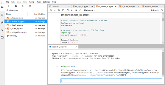

The development process is streamlined because sections of code (or cells) can be run iteratively while updating results and graphs. JupyterLab can be accessed from a web browser and supports a Python console with tab completions, tooltips, and visual output. One of the difficulties of using Jupyter notebooks with Kinetica in the past had been that environments needed to be installed with all the necessary dependencies. In this tutorial, the process will be simplified with a Docker image that integrates the components, so they can run locally on any Intel-based machine. The Docker image integrates the following major components:

JupyterLab
Kinetica 6.2
CentOS 7
Python 3.6

The Python environment has the necessary modules for:

Interaction with Kinetica using ODBC or the native API
Creating and executing Kinetica UDF’s
Execution of ML Models on Kinetica (e.g. Pandas, PyTorch, TensorFlow)

The Kinetica Intel build does not give GPU-accelerated performance and should be used for development purposes only.

Prerequisites

This tutorial requires the following:

Docker
Kinetica Developer Edition

Docker

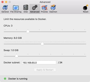
Docker can be downloaded from the Docker store:

Mac: https://store.docker.com/editions/community/docker-ce-desktop-mac
Linux: https://docs.docker.com/install/linux/docker-ce/centos/

After installing, select the Advanced preferences and allocate at least 6GB of memory for the VM as shown below.

Install

All the required code is available in the kinetica-jupyterlab Git repository:

https://github.com/kineticadb/kinetica-jupyterlab

You can use git clone to fetch a local copy.

git clone https://github.com/kineticadb/kinetica-jupyterlab
cd kinetica-jupyterlab

Setting Permissions

The two volumes that will be mounted in Docker, docker/share & notebooks, need to be writable by the image’s gpudb user, which has a uid of 1000. With some operating systems (osxfs), this is managed automatically by Docker. For others, the directories will need to be given permission directly. From the kinetica-jupyterlab directory, run the following:

chown -R 1000 docker/share notebooks

Entering the License Key

The database is configured to start automatically, but for this to succeed, a license key must be configured. Edit docker/share/conf/gpudb.conf, uncomment the line with license_key, and add the key:

# The license key to authorize running.
license_key = <license key>

If the key is invalid, the container will fail to start.

Pulling the Image

This section will demonstrate how to use docker-compose to pull the kinetica/kinetica-jupyterlab image from DockerHub. From the kinetica-jupyterlab directory, go into the docker directory and run docker-compose pull.

cd docker
docker-compose pull

The docker image command can be used to verify the download.

docker image list

Sample output:

REPOSITORY                     TAG                 IMAGE ID            CREATED             SIZE
kinetica/kinetica-jupyterlab   6.2                 e9702b6e31fb        28 minutes ago      7.35GB
centos                         7                   49f7960eb7e4        7 weeks ago         200MB

Managing the Container

This tutorial uses docker-compose to manage the parameters of the container. This can simplify the configuration process, as all of the settings are in the docker-compose.yml file.

Starting

Run the below docker-compose up command to start the image. The combined log output of Kinetica and JupyterLab will be displayed in the console. This console needs to be open for as long as the container is running. From the kinetica-jupyterlab/docker directory:

docker-compose up

Sample output:

Creating network "docker_default" with the default driver
Creating gpudb-jupyterlab-6.x ... done
Attaching to gpudb-jupyterlab-6.x
[...]
gpudb-jupyterlab-6.x | 2018-07-25 23:45:04.516 INFO  (2494,5923,r0/gpudb_sl_shtbl ) d0a1758a319b Utils/GaiaHTTPUtils.h:161 - JobId:1011; call_gaia_internal endpoint: /show/table completed in: 0.00193 s

Using

To use a Unix shell in the container, open up a separate console session and run the following from the kinetica-jupyterlab/docker directory:

docker-compose exec gpudb /bin/bash
su - gpudb

Stopping

To stop the container, use the docker-compose down command. From the kinetica-jupyterlab/docker directory:

docker-compose down

Sample output:

Stopping gpudb-jupyterlab-6.x ... done
Removing gpudb-jupyterlab-6.x ... done
Removing network docker_default

Exploring the Environment

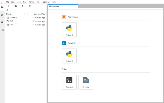
To access to GAdmin, open URL http://localhost:8080 and log in as an admin user (default username/password is admin/admin ). To access JupyterLab, open URL http://localhost:8888 and enter password kinetica. When logged in, the file browser will appear on the left.

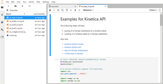
Navigate to the Examples folder, and open notebook ex_kapi_io.ipynb. This notebook demonstrates basic interactions between Pandas dataframes and Kinetica via the functions in the KIJO module.

Select Kernel -> Restart Kernel and Run All Cells… to clear the outputs. Then select the first cell and click the Play button to run each cell. Each notebook has a separate Python process or kernel that remembers the variables that were created when cells were executed. Cells can be modified and re-executed without starting from the beginning. A Python console can also be attached to the same kernel as a notebook. Right click on a cell and select New Console For Notebook. Enter one of the variables executed from the notebook (e.g. _test_df) and then press Shift+Enter to see the contents in the console.

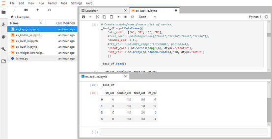
Use Tab for term completions and Shift+Tab for tooltips.

JupyterLab Contents

This repository contains an integrated environment that provides accelerated development of Kinetica-based ML Models. It makes use of CentOS 7, Kinetica, JupyterLab, and Python 3.6 for this purpose. JupyterLab has the following Python 3.6 libraries for integrating ML libraries with Kinetica:

It also has the following libraries for ML model development:

Example Notebooks are provided that demonstrate:

Connectivity between Pandas Dataframes and Kinetica with ODBC and the native API
ML models including an SVD recommender

Within the kinetica-jupyterlab directory, there are two directories of note:

docker - contains the scripts necessary to build and run the Docker image
notebooks - contains notebooks and Python scripts needed to run them; will be mounted inside the image and its contents will be visible in JupyterLab

Mounted Volumes

Host Location	Mount Point
kinetica-jupyterlab/docker/share	/opt/share
kinetica-jupyterlab/notebooks	/opt/notebooks

Example Notebooks

Example notebooks are located in notebooks/Examples, which document and demonstrate interaction of JupyterLab with Kinetica.

Notebook File	Description
ex_kapi_io.ipynb	Load/Save Pandas Dataframes with the Kinetica REST API
ex_kodbc_io.ipynb	Load/Save Pandas Dataframes with the Kinetica ODBC
ex_kudf_io.ipynb	Create/Execute a UDF to calculate sum-of-squares
ex_kudf_lr.ipynb	Create/Execute a UDF to calculate linear regression with distributed inferencing
ex_widget_lorenz.ipynb	Example of real-time refresh of calculation with widgets

SVD Recommender and Visualization Example

The following set of notebooks contain an example of how to use SVD with Kinetica to build a recommender engine. The notebooks generate result tables and must be executed in-order.

Notebook	Description
svd_1_ingest.ipynb	Download and ingest Amazon rating data
svd_2_calc.ipynb	Calculate SVD matrices and save results
svd_3_recommend.ipynb	Demonstration of a recommender
svd_4_visualization.ipynb	Clustering and visualization with SVD

KJIO Utility Library

A set of utility functions collectively called Kinetica Jupyter I/O are located in notebooks/KJIO to simplify the task of interacting with Kinetica from notebooks. The example notebooks demonstrate their functionality.

Script	Description
kapi_io.py	Loads and saves Dataframes to/from Kinetica tables
kmodel_io.py	Loads and saves ML models with a Kinetica table
kodbc_io.py	Interacts with tables using ODBC
kudf_io.py	Functions that simplify creation and execution of UDFs

Conclusion

The JupyterLab environment integrates many components. With it, external datasources can be ingested, the data analyzed with some of the most powerful ML libraries, the results saved to Kinetica, the data further processed with UDFs, and each step visualized, all in a single notebook. Use cases can have documentation and equations added to aid in telling a data-driven story to multiple audiences.

References

Additional online resources are available here:

​Introduction

​Prerequisites

​Docker

​Install

​Setting Permissions

​Entering the License Key

​Pulling the Image

​Managing the Container

​Starting

​Using

​Stopping

​Exploring the Environment

​JupyterLab Contents

​Mounted Volumes

​Example Notebooks

​SVD Recommender and Visualization Example

​KJIO Utility Library

​Conclusion

​References

Introduction

Prerequisites

Docker

Install

Setting Permissions

Entering the License Key

Pulling the Image

Managing the Container

Starting

Using

Stopping

Exploring the Environment

JupyterLab Contents

Mounted Volumes

Example Notebooks

SVD Recommender and Visualization Example

KJIO Utility Library

Conclusion

References