

Prerequisites
- KiSQL (if running the SQL examples)
- Python API (if running the Python examples)
- Sample CSV data files, which should be downloaded & copied to the host running the SQL client. The data files can be downloaded here:
Loading Sample Data
Data loading will be done via SQL. First log in to the database:Create Geospatial Example Schema
Create NYC Neighborhood Shape Table
Create NYC Taxi Trip Table
Create NYC Taxi Zone Shape Table
Create KiFS Directory for Geospatial Data Files
Stage NYC Neighborhood Data
Load NYC Neighborhood Data
Stage NYC Taxi Trip Data
Load NYC Taxi Trip Data
Stage NYC Taxi Zone Data
Load NYC Taxi Zone Data
Examples via SQL
Creating a Table and Inserting WKT Data
First, a points-of-interest table is created and loaded with sample WKT data.Create POI Table
Populate POI Table
Scalar Functions
For the complete list of scalar functions, see both Scalar Functions and Enhanced Performance Scalar Functions.GEODIST Example
ST_AREA Example
Aggregation Functions
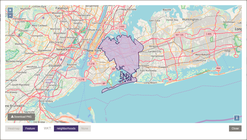
For the complete list of aggregation functions, see Aggregation Functions.ST_DISSOLVE Example
Joins
Many geospatial/geometry functions can be used to join data sets. For the complete list of join and other scalar functions, see both Scalar Functions and Enhanced Performance Scalar Functions.Implicit Geospatial Containment Join
Explicit Geospatial Intersection Join
Explicit Geospatial Intersection Join with Geospatial Aggregation
Equality
There are three ways of checking if two geometries are equal, which each have different thresholds:ST_EQUALS()ST_ALMOSTEQUALS()ST_EQUALSEXACT()
Equality Comparisons Between Two Points
Examples via the Python API
Creating a Table and Inserting WKT Data
First, a points-of-interest table is created and loaded with sample WKT data.Create POI Table
Populate POI Table
Scalar Functions
For the complete list of scalar functions, see both Scalar Functions and Enhanced Performance Scalar Functions.GEODIST Example
ST_AREA Example
Aggregation Functions
For the complete list of aggregation functions, see Aggregation Functions.ST_DISSOLVE Example
Joins
Many geospatial/geometry functions can be used to join data sets. For the complete list of join and other scalar functions, see both Scalar Functions and Enhanced Performance Scalar Functions.Implicit Geospatial Containment Join
Implicit Geospatial Intersection Join
Implicit Geospatial Intersection Join with Geospatial Aggregation
Equality
There are three ways of checking if two geometries are equal, which each have different thresholds:ST_EQUALS()ST_ALMOSTEQUALS()ST_EQUALSEXACT()
Equality Comparisons Between Two Points
Complete Samples
Included below are complete examples containing all the above requests and the output.- Python (see Python Developer Guide for configuration & execution details)
- SQL (see ODBC/JDBC Connector for configuration & execution details)