Backhaul Routing in Python

The following is a complete example, using the Python API, of solving a graph created with Seattle road network data for a backhaul routing problem via the /solve/graph endpoint. For more information on Graphs & Solvers, see Graphs & Solvers Concepts.

Prerequisites

The prerequisites for running the backhaul routing solve graph example are listed below:

Graph server enabled
Python API
Solve graph script
Seattle road network CSV file

Python API Installation

Depending on the target operating system, a Python virtual environment may need to be installed first:

Python Virtual Environment

The native Kinetica Python API is accessible through the following means:

PyPI
Git

Python Virtual Environment

A Python virtual environment is necessary to install in an operating environment where Python is externally managed.

Install a Python virtual environment:
python3 -m venv .venv
Activate the Python virtual environment:
source .venv/bin/activate

PyPI

Install the API:
pip3 install gpudb
Test the installation:
python3 -c "import gpudb;print('Import Successful')"
If Import Successful is displayed, the API has been installed as is ready for use.

Git

In the desired directory, run the following, but be sure to replace <kinetica-version> with the name of the installed Kinetica version, e.g., v7.2:
git clone -b release/<kinetica-version> --single-branch https://github.com/kineticadb/kinetica-api-python.git
Change directory into the newly downloaded repository:
cd kinetica-api-python
In the root directory of the unzipped repository, install the Kinetica API:
sudo pip3 install .
Test the installation (Python3 is necessary for running the API example):
python3 examples/example.py

Data File

The example script references the road_weights.csv data file, mentioned in the Prerequisites, in the current local directory, by default. This directory can specified as a parameter when running the example script.

Script Detail

This example is going to demonstrate solving for routing a given set of remote assets, e.g., stores, to a number of fixed assets, e.g, distribution centers, located in a Seattle road network.

Constants

SCHEMA — the name of the schema in which the tables supporting the graph creation and match operations will be created
The schema is created during the table setup portion of the script because the schema must exist prior to creating the tables that will later support the graph creation and match operations.
TABLE_SRN — the name of the table into which the Seattle road network dataset is loaded
GRAPH_S — the Seattle road network graph
TABLE_GRAPH_S_BSOLVED — the solved Seattle road network graph using the BACKHAUL_ROUTING solver type

Constant Definitions

SCHEMA = "graph_s_backhaul"
TABLE_SRN = SCHEMA + ".seattle_road_network"

GRAPH_S = SCHEMA + ".seattle_road_network_graph"
TABLE_GRAPH_S_BSOLVED = GRAPH_S + "_backhaul_routing_solved"

Graph Creation

One graph is used for the backhaul solve graph example utilized in the script: seattle_road_network_graph, a graph based on the road_weights dataset (the CSV file mentioned in Prerequisites). The seattle_road_network_graph graph is created with the following characteristics:

It is directed because the roads in the graph have directionality (one-way and two-way roads)
It has no explicitly defined nodes because the example relies on implicit nodes attached to the defined edges
The edges are identified by WKTLINE, using WKT LINESTRINGs from the WKTLINE column of the seattle_road_network table. The road segments’ directionality (DIRECTION) is derived from the TwoWay column of the seattle_road_network table.
The weights (VALUESPECIFIED) are represented using the time taken to travel the segment found in the time column of the seattle_road_network table. The weights are matched to the edges using the same WKTLINE column as edges (EDGE_WKTLINE) and the same TwoWay column as the edge direction (EDGE_DIRECTION).
It has no inherent restrictions for any of the nodes or edges in the graph
It will be replaced with this instance of the graph if a graph of the same name exists (recreate)

Create Seattle Road Network Graph

create_s_graph_response = kinetica.create_graph(
    graph_name = GRAPH_S,
    directed_graph = True,
    nodes = [],
    edges = [
        TABLE_SRN + ".WKTLINE AS WKTLINE",
        TABLE_SRN + ".TwoWay AS DIRECTION"
    ],
    weights = [
        TABLE_SRN + ".WKTLINE AS EDGE_WKTLINE",
        TABLE_SRN + ".TwoWay AS EDGE_DIRECTION",
        TABLE_SRN + ".time AS VALUESPECIFIED"
    ],
    restrictions = [],
    options = {
        "recreate": "true"
    }
)

Backhaul Routing

First, the fixed assets and remote assets are set.

Define Fixed Asset Locations

fixed_assets = [
    "POINT(-122.37694377950754 47.69058183874783)",
    "POINT(-122.37591381124582 47.6947415132984)",
    "POINT(-122.3635541921052 47.70005617015495)",
    "POINT(-122.35565776876535 47.70583235665686)",
    "POINT(-122.35531444601145 47.72477375603093)",
    "POINT(-122.33540172628489 47.72361898977214)",
    "POINT(-122.32407207540598 47.72408089934756)",
    "POINT(-122.32647533468332 47.73562730759159)",
    "POINT(-122.32922191671457 47.74209217807247)",
    "POINT(-122.31205577901926 47.741399551774876)",
    "POINT(-122.31274242452707 47.737705389219734)",
    "POINT(-122.29935283712473 47.73701270455902)",
    "POINT(-122.2976362233552 47.73262548770682)",
    "POINT(-122.2921430592927 47.73354914302527)",
    "POINT(-122.29179973653879 47.72200227400312)",
    "POINT(-122.30003948263254 47.712531931184785)",
    "POINT(-122.30278606466379 47.701442513285734)",
    "POINT(-122.30518932394114 47.694048257248284)",
    "POINT(-122.30244274190989 47.68827076507089)",
    "POINT(-122.31514568380442 47.68480396253861)",
    "POINT(-122.32750530294504 47.68711518982914)",
    "POINT(-122.3474180226716 47.687577422998146)",
    "POINT(-122.37763042501535 47.686421832395006)",
    "POINT(-122.37694377950754 47.69058183874783)"
]
remote_assets = [
    "POINT(-122.324612 47.725231)", "POINT(-122.362112 47.696131)",
    "POINT(-122.356212 47.741731)", "POINT(-122.341512 47.702631)",
    "POINT(-122.327412 47.737131)", "POINT(-122.344912 47.727531)",
    "POINT(-122.291612 47.657631)", "POINT(-122.324512 47.703831)",
    "POINT(-122.297712 47.731231)", "POINT(-122.317912 47.699431)",
    "POINT(-122.351412 47.713731)", "POINT(-122.295612 47.670531)",
    "POINT(-122.321812 47.672731)", "POINT(-122.295612 47.697531)",
    "POINT(-122.333012 47.689831)", "POINT(-122.298812 47.711731)",
    "POINT(-122.309612 47.684931)", "POINT(-122.359712 47.716431)",
    "POINT(-122.360612 47.659231)", "POINT(-122.299012 47.707431)",
    "POINT(-122.311612 47.666831)", "POINT(-122.315912 47.724631)",
    "POINT(-122.316912 47.709531)", "POINT(-122.313212 47.685731)",
    "POINT(-122.321712 47.721231)", "POINT(-122.339512 47.695031)",
    "POINT(-122.310512 47.692531)", "POINT(-122.326512 47.679731)",
    "POINT(-122.358112 47.705731)", "POINT(-122.352812 47.715931)",
    "POINT(-122.291612 47.677531)", "POINT(-122.295712 47.666731)",
    "POINT(-122.303712 47.681531)", "POINT(-122.362312 47.732231)",
    "POINT(-122.347712 47.740431)", "POINT(-122.343512 47.685231)",
    "POINT(-122.326412 47.730631)", "POINT(-122.357812 47.670031)",
    "POINT(-122.321012 47.694531)", "POINT(-122.353312 47.737131)",
    "POINT(-122.323412 47.679031)", "POINT(-122.351012 47.701731)",
    "POINT(-122.349112 47.735931)", "POINT(-122.361612 47.675031)",
    "POINT(-122.320912 47.701931)", "POINT(-122.345412 47.693331)",
    "POINT(-122.357112 47.669631)", "POINT(-122.352912 47.685131)",
    "POINT(-122.361712 47.681331)", "POINT(-122.346312 47.722231)"
]

Next, the graph is solved with the solve results being exported to the response. The fixed assets are provided for the source nodes and the remote assets are provided for the destination nodes. All assets are snapped to corresponding locations on the Seattle road network graph.

Solve Graph

kinetica.solve_graph(
    graph_name = GRAPH_S,
    solver_type = "BACKHAUL_ROUTING",
    source_nodes = fixed_assets,
    destination_nodes = remote_assets,
    solution_table = TABLE_GRAPH_S_BSOLVED
)

The cost for each remote asset to travel to the nearest fixed asset is output:

Solve Graph Results

+--------------------------------------------+--------------------------------------------+---------------------+
| Remote Asset                               | Fixed Asset                                |   Cost (in seconds) |
|--------------------------------------------+--------------------------------------------+---------------------|
| POINT (-122.362029254436 47.6960599422455) | POINT (-122.363370358944 47.6996996998787) |            53.3698  |
| POINT (-122.357080578804 47.6691091060638) | POINT (-122.361868321896 47.674181163311)  |            87.0141  |
| POINT (-122.361868321896 47.674181163311)  | POINT (-122.361479401588 47.6807391643524) |            77.5143  |
| POINT (-122.360798120499 47.6589596271515) | POINT (-122.357080578804 47.6691091060638) |           136.192   |
| POINT (-122.357898652554 47.66950070858)   | POINT (-122.357080578804 47.6691091060638) |            17.3271  |
| POINT (-122.352880239487 47.7159807085991) | POINT (-122.355570495129 47.724609375)     |            77.6373  |
| POINT (-122.353100180626 47.7369394898415) | POINT (-122.355570495129 47.724609375)     |            91.7304  |
| POINT (-122.358089089394 47.7051097154617) | POINT (-122.355468571186 47.7056005597115) |            33.3519  |
| POINT (-122.351249456406 47.7014511823654) | POINT (-122.355468571186 47.7056005597115) |            55.9931  |
| POINT (-122.355599999428 47.7413892745972) | POINT (-122.353100180626 47.7369394898415) |            69.2636  |
| POINT (-122.361538410187 47.7329590916634) | POINT (-122.353100180626 47.7369394898415) |            75.0526  |
| POINT (-122.347639203072 47.7389994263649) | POINT (-122.353100180626 47.7369394898415) |            57.435   |
| POINT (-122.351528406143 47.7123489975929) | POINT (-122.352880239487 47.7159807085991) |            37.4391  |
| POINT (-122.359548211098 47.7159914374352) | POINT (-122.352880239487 47.7159807085991) |            58.7806  |
| POINT (-122.345010638237 47.7222892642021) | POINT (-122.352880239487 47.7159807085991) |            85.3496  |
| POINT (-122.361479401588 47.6807391643524) | POINT (-122.352418899536 47.6847597956657) |           104.085   |
| POINT (-122.341939508915 47.7014109492302) | POINT (-122.351249456406 47.7014511823654) |            68.9019  |
| POINT (-122.34799861908 47.735960483551)   | POINT (-122.347639203072 47.7389994263649) |            40.7816  |
| POINT (-122.34178930521 47.6854893565178)  | POINT (-122.347258329391 47.6876699924469) |            60.074   |
| POINT (-122.347250282764 47.6934716105461) | POINT (-122.347258329391 47.6876699924469) |            63.6802  |
| POINT (-122.352418899536 47.6847597956657) | POINT (-122.347258329391 47.6876699924469) |            79.6751  |
| POINT (-122.339128553867 47.6945605874062) | POINT (-122.347250282764 47.6934716105461) |            67.2841  |
| POINT (-122.345048189163 47.7268999814987) | POINT (-122.345010638237 47.7222892642021) |            38.4461  |
| POINT (-122.333168685436 47.6886409521103) | POINT (-122.327640652657 47.6872113347054) |            74.8597  |
| POINT (-122.327418029308 47.738299369812)  | POINT (-122.324389815331 47.7296707034111) |            39.7206  |
| POINT (-122.325079143047 47.7306604385376) | POINT (-122.324389815331 47.7296707034111) |            62.1762  |
| POINT (-122.324389815331 47.7296707034111) | POINT (-122.32419937849 47.7231100201607)  |            32.0087  |
| POINT (-122.320849299431 47.7212592959404) | POINT (-122.32419937849 47.7231100201607)  |            43.3122  |
| POINT (-122.321809530258 47.6730009913445) | POINT (-122.323319613934 47.6787811517715) |           119.879   |
| POINT (-122.326119840145 47.6790305972099) | POINT (-122.323319613934 47.6787811517715) |            25.2642  |
| POINT (-122.31192022562 47.666429579258)   | POINT (-122.321809530258 47.6730009913445) |           153.608   |
| POINT (-122.324620485306 47.7034413814545) | POINT (-122.320428192616 47.7022102475166) |            78.6723  |
| POINT (-122.31763869524 47.6994609832764)  | POINT (-122.320310175419 47.6949307322502) |            80.0134  |
| POINT (-122.317858636379 47.7097713947296) | POINT (-122.31763869524 47.6994609832764)  |           110.156   |
| POINT (-122.320428192616 47.7022102475166) | POINT (-122.31763869524 47.6994609832764)  |            52.7903  |
| POINT (-122.31330960989 47.6850092411041)  | POINT (-122.314240336418 47.6848804950714) |            14.4332  |
| POINT (-122.323319613934 47.6787811517715) | POINT (-122.314240336418 47.6848804950714) |           101.485   |
| POINT (-122.309948801994 47.6848509907722) | POINT (-122.31330960989 47.6850092411041)  |            24.6041  |
| POINT (-122.315238118172 47.7250197529793) | POINT (-122.312869727612 47.73756980896)   |           155.957   |
| POINT (-122.303929924965 47.6812407374382) | POINT (-122.309948801994 47.6848509907722) |            91.3501  |
| POINT (-122.320310175419 47.6949307322502) | POINT (-122.309519648552 47.6921412348747) |           113.515   |
| POINT (-122.309519648552 47.6921412348747) | POINT (-122.305528521538 47.6939195394516) |            48.0132  |
| POINT (-122.291640043259 47.675801217556)  | POINT (-122.303929924965 47.6812407374382) |           136.551   |
| POINT (-122.293268144131 47.6975002884865) | POINT (-122.302768528461 47.7011802792549) |           104.879   |
| POINT (-122.299528419971 47.7120405435562) | POINT (-122.30034917593 47.7120512723923)  |             7.42232 |
| POINT (-122.299359440804 47.7075102925301) | POINT (-122.299528419971 47.7120405435562) |            48.3775  |
| POINT (-122.297900319099 47.7301615476608) | POINT (-122.296540439129 47.732709646225)  |            42.6013  |
| POINT (-122.29111969471 47.6586404442787)  | POINT (-122.295649945736 47.6663303375244) |            88.8346  |
| POINT (-122.295649945736 47.6663303375244) | POINT (-122.295430004597 47.6703295111656) |            50.3047  |
| POINT (-122.295430004597 47.6703295111656) | POINT (-122.291640043259 47.675801217556)  |            79.9073  |
+--------------------------------------------+--------------------------------------------+---------------------+

The solution output to WMS:

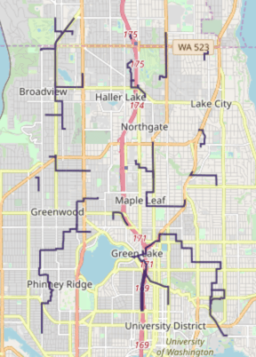
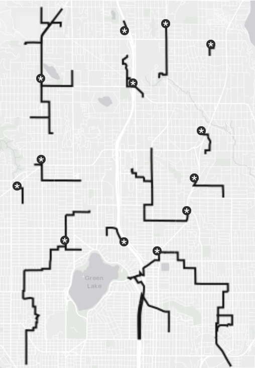
To demonstrate how the remote assets are routed back to the fixed assets, the fixed assets can be plotted using a separate WMS call and mapped together with the solution. The picture below represents this; the fixed assets are * icons while remote assets can be found in lines leading away from the fixed assets.

Download & Run

Included below is a complete example containing all the above requests, the data files, and output.

To run the complete sample, ensure that:

the solve_graph_seattle_backhaul.py script is in the current directory
the road_weights.csv file is in the current directory or use the data_dir parameter to specify the local directory containing it

Then, run the following:

Run Example

python solve_graph_seattle_backhaul.py [--url <kinetica_url>] --username <username> --password <password> [--data_dir <data_file_directory>]

​Prerequisites

​Python API Installation

​Python Virtual Environment

​PyPI

​Git

​Data File

​Script Detail

​Constants

​Graph Creation

​Backhaul Routing

​Download & Run

Prerequisites

Python API Installation

Python Virtual Environment

PyPI

Git

Data File

Script Detail

Constants

Graph Creation

Backhaul Routing

Download & Run