Data
All the data in the database can be viewed through the Data menu selection. From here, you can view detailed information about each table or collection; use WMS to generate a heatmap of a table with geocoordinates; create, delete, or configure a table; or import data.
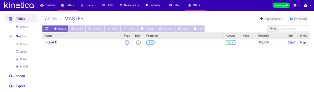
Tables
The Tables page lists all tables and schemas/collections in the database in a grid layout. Also available are the object type (table or collection), type of distribution (replicated, sharded, or neither), feature set (see list below), global access rights (read/write), keys (primary, shard, and foreign) and associated columns, and the record count.
The types of features are as follows:
- PERS (PERSISTED) -- the table exists on disk & in memory (i.e., not memory-only) and will exist across database restarts
- JOIN -- this is a join view
- RESU (RESULT_TABLE) -- results from endpoint operations like Create Projection and Create Union
- VIEW -- this table is a filtered data view or materialized view
From this page, the following functionality is available:
 (Refresh) -- refresh all tables
- Create -- create a new table
- Config -- modify the selected table
- Rename -- rename the selected table
- Move -- move the selected table(s) or view(s) to a different collection
- Delete -- delete the selected table(s)
- Rebuild -- rebuild the selected table(s) and/or collection(s)
- Memory -- display the current amount of used memory for the selected table(s); if a collection is selected, the child tables' memory will be displayed
- Stats -- display statistics regarding a selected column or all columns in the table, e.g., estimated cardinality, mean value, standard deviation, etc., and recommendations for improving the structure of the table, e.g., dictionary encoding, smaller column type, etc.
- Sec -- manage row- and column- security for the selected table
- Filter -- only display tables matching the given search text
- Sync Mode -- if enabled, table row counts will be accurate but potentially slow
- + Add Collection -- specify a name, then create a collection
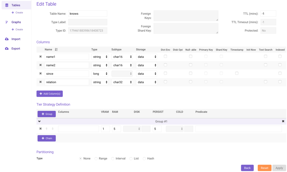
Configuring
To configure an existing table, click Config, update the table configuration as necessary, and click Apply. Click Reset to discard any pending modifications.
Allowed modifications include:
- Renaming the table
- Modifying the TTL
- Renaming the non-primary/shard key columns
- Modifying the type, subtype, storage, and properties of a non-primary/ shard key column
- Removing any non-primary/shard key columns
- Adding new columns
- Adjusting the tier strategy definition
- Adjusting the table partitioning
Defining a Tier Strategy
From the Edit Table page:
Click + Group to append additional column strategy groupings to the table
Click + Chain to append additional priority definitions to a group
Provide a comma-separated list of columns, an eviction priority for each available tier (tiers are defined in
/opt/gpudb/core/etc/gpudb.conf), and an optional predicateTip
Omit Columns to apply the strategy to the entire table
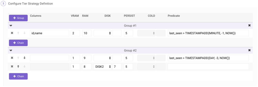
Example
For instance, consider the following tier strategy, applied to a table with a
timestamp column named last_seen, a positive integer id column, and a
string name column:
(
    (VRAM 1, RAM 9) WHERE last_seen > TIMESTAMPADD(DAY, -3, NOW()),
    (VRAM 1, RAM 8, DISK2 7)
),
(
    COLUMNS id, name
        (VRAM 2, RAM 10) WHERE last_seen > TIMESTAMPADD(MINUTE, -1, NOW())
)
To recreate this strategy in the table configuration interface:
Partitioning
From the Edit Table page:
- Select a partition type.
- Provide as many Key(s) as necessary. Click + to add key expressions.
- Provide as many Definition(s) as necessary. Click + to add definitions.
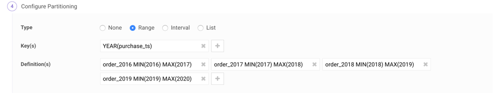
Example
To create a range-partitioned table with the following criteria:
- partitioned by the date/time of the order
- partitions for years 2016, 2017, 2018, & 2019
- records not in that range go to the default partition
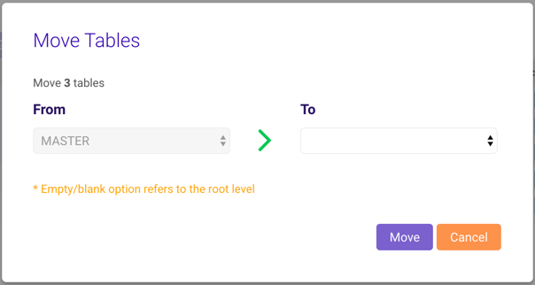
Moving
To move a table to another collection, select a table (or tables) then click Move. Select which collection to move the table(s) to (the blank option is the root-level collection) and click Move.
Deleting
To delete a table, select a table (avoid clicking the table's name, as it will open the Data Grid page) then click Delete and confirm the deletion of the selected table.
Rebuilding
To rebuild a table or collection if you are unable to query it, select a table(s) or collection(s), click Rebuild, then confirm the rebuild. Acknowledge the warning, then the selected table(s) and/or collection(s) will be rebuilt. For more information on rebuilding the database, see Admin.
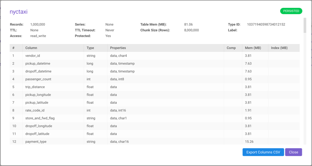
Detailed Table Information
To view table, schema, memory usage, and tier strategy information, click Detail in the Info column. The column grid can be exported to CSV by clicking Export CSV.
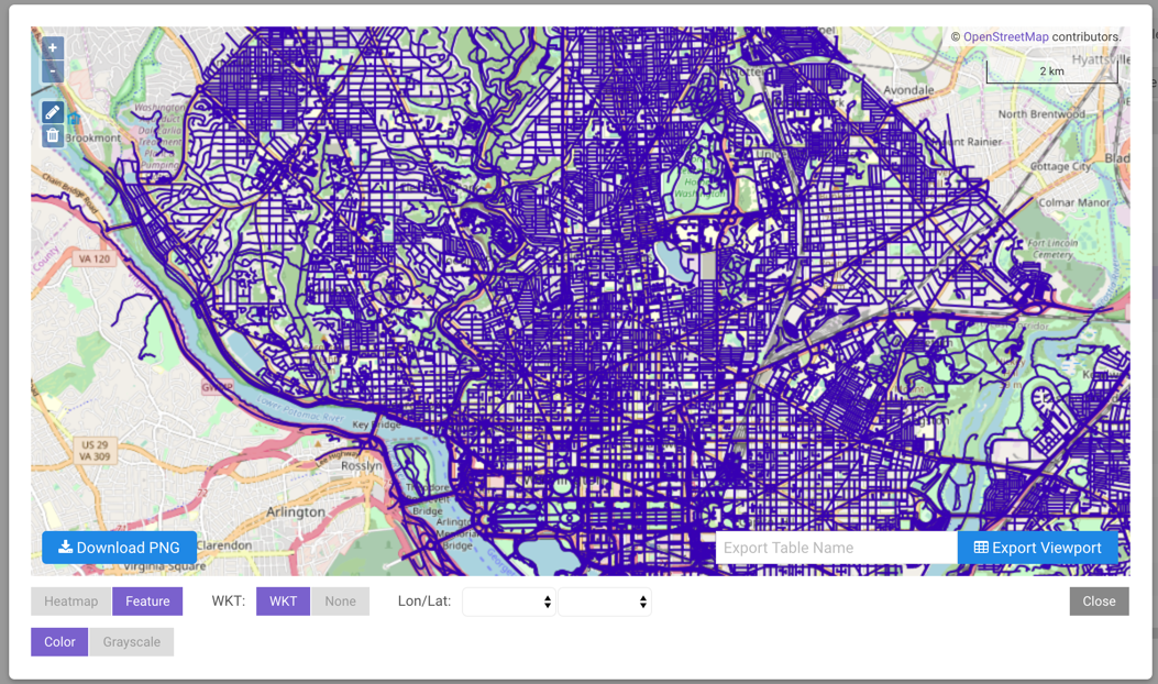
WMS
If your data contains coordinates and/or geometry data, you can:
- When viewing the list of tables (), click the Map link in the WMS column
- When browsing a table's datagrid, click the WMS button in the top bar
You can use the + / - on the left or the scroll wheel
of your mouse to zoom in and out of an area. Click  to draw a polygon on
top of the map; this will act as a filter for the viewport. Click
to draw a polygon on
top of the map; this will act as a filter for the viewport. Click  to
remove any polygons on the map. Click Download PNG to download a
to
remove any polygons on the map. Click Download PNG to download a
.png file of the current viewport. Provide a table name and click
Export Viewport to export the points in the current viewport to
a separate table; note that if any polygon(s) were drawn on the
map, only the points inside those polygons will be exported to the new table.
Note
The map will default to Heatmap mode. To render full WKT geometry, click Feature. Whilst rendering features, click a feature on the map to display additional information about the feature.
The following column types can be used to populate the map with latitude/longitude points (assuming the columns being used to render the points are of the same type):
doublefloatintint16int8longtimestamp(the raw epoch value will be used to render the point)decimal
The following column types can be used to populate the map with WKT objects:
wktwkb
If there are multiple WKT/WKB columns, select the desired column to display, select None to not display any compatible column(s), or select All to display all compatible column(s) next to WKT; if there are multiple longitude / latitude columns, select the desired columns from the Lon/Lat drop-down menus. If there are both WKT objects and longitude / latitude points present in a table, select the WKT column to display WKT or select None and the desired columns from the Lon/Lat drop-down menus to display longitude / latitude points.
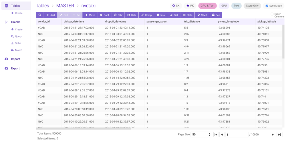
Data Grid
To view the individual records in a table, click the table name. This will display the data grid page. From here, the following functionality is available:
- (Refresh) -- refresh the table
- Add -- insert a new record
- Edit -- modify the selected record
- Delete -- delete the selected record
- Move -- move the table or view to a different collection
- Conf -- modify the table or view
- CSV -- export data to CSV
- Hide -- hide displayed columns within the grid
- Comp -- compress individual columns of data in memory; see Compression for details
- Info -- display table detail
- Dist -- display cross-node data distribution graph
- Stats -- display statistics regarding a selected column or all columns in the table, e.g., estimated cardinality, mean value, standard deviation, etc., and recommendations for improving the structure of the table, e.g., dictionary encoding, smaller column type, etc.
- WMS -- plot data from tables with geospatial data on a map
- Sec -- manage row- and column- security for the table
- Sync Mode -- if enabled, table row counts will be accurate but potentially slow
Export Data
From the data grid page, select CSV. You will have the option to export all of the data or records within a range, specify the type of header, and how to order the data on export.
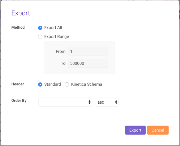
Once you click the Export button, the data will be downloaded to your computer. The standard header is just a comma-delimited list of column header names:

The Kinetica Schema is a comma-delimited list of column headers with bar-delimited column properties:

Note
Null values are represented as \N. This can be changed by
modifying the data_file_string_null_value parameter in
/opt/gpudb/tomcat/webapps/gadmin/WEB-INF/classes/gaia.properties.
Compression
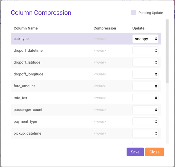
In addition to using the API or SQL to set compression, you can set it by clicking Comp on the data grid page, opening up the Column Compression dialog. Each column will be shown with its current compression setting under Compression and a selectable new compression setting under Update. After compression adjustments have been made, click Save to put those changes into effect. See Compression for more detail on compression and compression types.
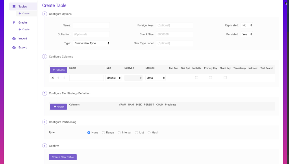
Creating
A table can be created by clicking Create (underneath Tables) on the left menu to navigate to the Create Table page. After configuring the name, containing collection name, distribution scheme, keys, column set, tier strategy definition, and partitioning, click Create New Table.
Advanced Table Security
Advanced table security (e.g., row- and column-level) can be enabled on a per-table basis for select users and roles by:
- When viewing the list of tables (), select a table then click the Sec button in the top bar
- When browsing a table's datagrid, click the Sec button in the top bar
A user or role must have the table_read permission on a selected table for
the row- and/or column-level security to apply. Review
Row-Level Security and Column-Level Security for
more information.
Important
Advanced Table Security can only be accessed by users with the
system_admin permission.
Users
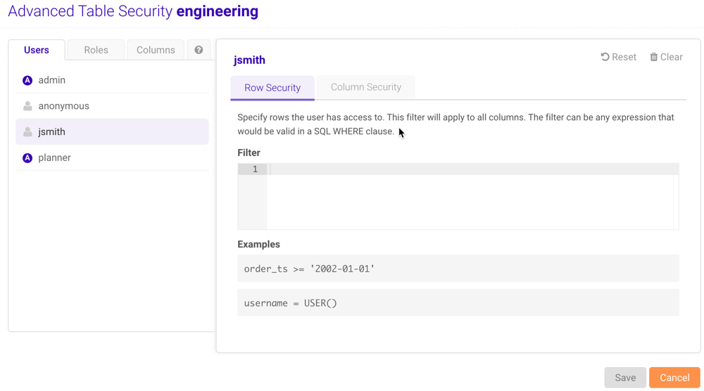
Individual users can have row- and column-level security imposed on them, restricting or granting access to particular data. To apply security to a user:
Navigate to the Advanced Table Security window and display the Users tab.
Select a user from the list.
Note
Row- and column-level security cannot be configured for users with the
system_adminpermission.Apply Row Security and Column Security as necessary.
To apply Row Security:
- Click the Row Security tab.
- Provide a valid SQL
WHERE-like expression in the Filter text field. This filter will apply to all columns.
To apply Column Security:
Click the Column Security tab.
Select a column from the drop-down menu.
Click Add Column.
Optionally, if the column is a fixed-width
stringcolumn, select a Transform option:- Mask -- the column value will be masked after some length,
for some width of characters, with a select character. If no mask
exists for the column currently, one must be defined. Click
 to
jump to the Columns tabe and define one. See
Columns for more information.
to
jump to the Columns tabe and define one. See
Columns for more information. - Obfuscate -- each unique original column value will be exchanged for a unique non-negative number
Important
Review Column-Level Security for more information on masking and obfuscation.
- Mask -- the column value will be masked after some length,
for some width of characters, with a select character. If no mask
exists for the column currently, one must be defined. Click
Optionally, apply a valid SQL
WHERE-like expression in the Filter text field.Repeat the previous steps for as many columns as necessary.
Click Save and confirm the update for the selected user.
Tip
Click Reset to reset the modified security settings to the previously saved settings. Click Clear to remove any saved settings.
Roles
Individual roles can have row- and column-level security imposed on them, restricting or granting access to particular data. To apply security to a role:
Navigate to the Advanced Table Security window and display the Roles tab.
Select a role from the list.
Note
Row- and column-level security cannot be configured for roles with the
system_adminpermission.Apply Row Security and Column Security as necessary.
To apply Row Security:
- Click the Row Security tab.
- Provide a valid SQL
WHERE-like expression in the Filter text field. This filter will apply to all columns.
To apply Column Security:
Click the Column Security tab.
Select a column from the drop-down menu.
Click Add Column.
Optionally, if the column is a fixed-width
stringcolumn, select a Transform option:- Mask -- the column value will be masked after some length,
for some width of characters, with a select character. If no mask
exists for the column currently, one must be defined. Click to
jump to the Columns tabe and define one. See
Columns for more information.
- Obfuscate -- each unique original column value will be exchanged for a unique non-negative number
Important
Review Column-Level Security for more information on masking and obfuscation.
- Mask -- the column value will be masked after some length,
for some width of characters, with a select character. If no mask
exists for the column currently, one must be defined. Click
Optionally, apply a valid SQL
WHERE-like expression in the Filter text field.Repeat the previous steps for as many columns as necessary.
Click Save and confirm the update for the selected role.
Tip
Click Reset to reset the modified security settings to the previously saved settings. Click Clear to remove any saved settings.
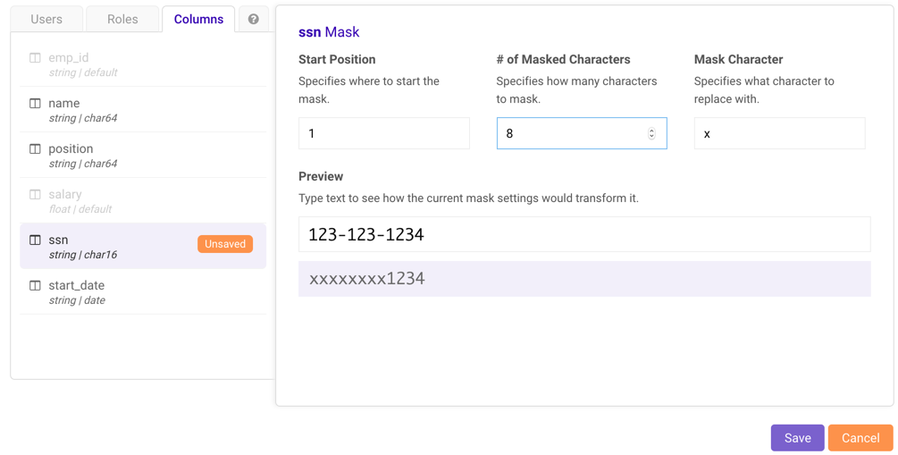
Columns
Fixed-width string columns in the selected table can have pre-configured
masks applied when setting column-level security for a user or role. To create a
mask for a column:
- Navigate to the Advanced Table Security window and display the Columns tab.
- Select a valid column from the list.
- Specify a Start Position for the mask.
- Specify the # of Masked Characters.
- Specify the Mask Character.
- Optionally, type into the Preview field to preview the mask before saving.
- Click Save and confirm the column mask.
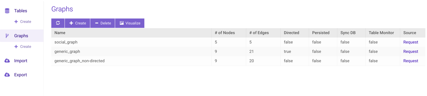
Graphs
The Graphs page displays any created graphs as well as various information and statistics about each graph. Click Request under Source to see the JSON used to create the graph as it is. Click Create to open the Create Graph interface. Click a graph then click Delete to delete the graph. Click Visualize to use WMS to display the graph. Consult Network Graphs & Solvers Concepts for more information on graphs.
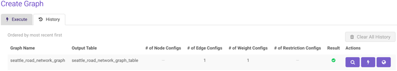
Tip
On any of the interfaces described below, click History to
view previous requests made to that particular interface, view details
about each request, reload a request, or view WMS for the request (if
Enable Graph Draw was set to True)
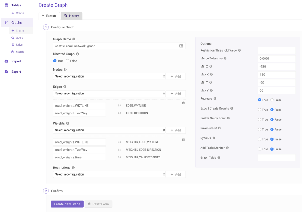
Create
A graph can be created by clicking Create (underneath Graphs) on the left menu to navigate to the Create Graph page. Follow the steps below to create a graph using the interface:
Important
It's highly recommended you consult Network Graphs & Solvers Concepts and /create/graph for information on identifiers, valid configurations, combinations, and graph options before creating a graph with GAdmin.
- Provide a name for the graph.
- Choose whether the graph should be directed
- Optionally, select a desired node configuration from the Nodes drop-down menu and click Add +. For each identifier that appears after adding the configuration to the graph, provide a column name, expression, or raw value (as outlined in Components and Identifiers) to use with the identifier. Repeat as necessary.
- Select a desired edge configuration from the Edges drop-down menu and click Add +. For each identifier that appears after adding the configuration to the graph, provide a column name, expression, or raw value (as outlined in Components and Identifiers) to use with the identifier. Repeat as necessary.
- Select a desired weight configuration from the Weights drop-down menu and click Add +. For each identifier that appears after adding the configuration to the graph, provide a column name, expression, or raw value (as outlined in Components and Identifiers) to use with the identifier. Repeat as necessary.
- Optionally, select a desired restriction configuration from the Restrictions drop-down menu and click Add +. For each identifier that appears after adding the configuration to the graph, provide a column name, expression, or raw value (as outlined in Components and Identifiers) to use with the identifier. Repeat as necessary.
- Adjust the options as desired.
- Click Create New Graph.
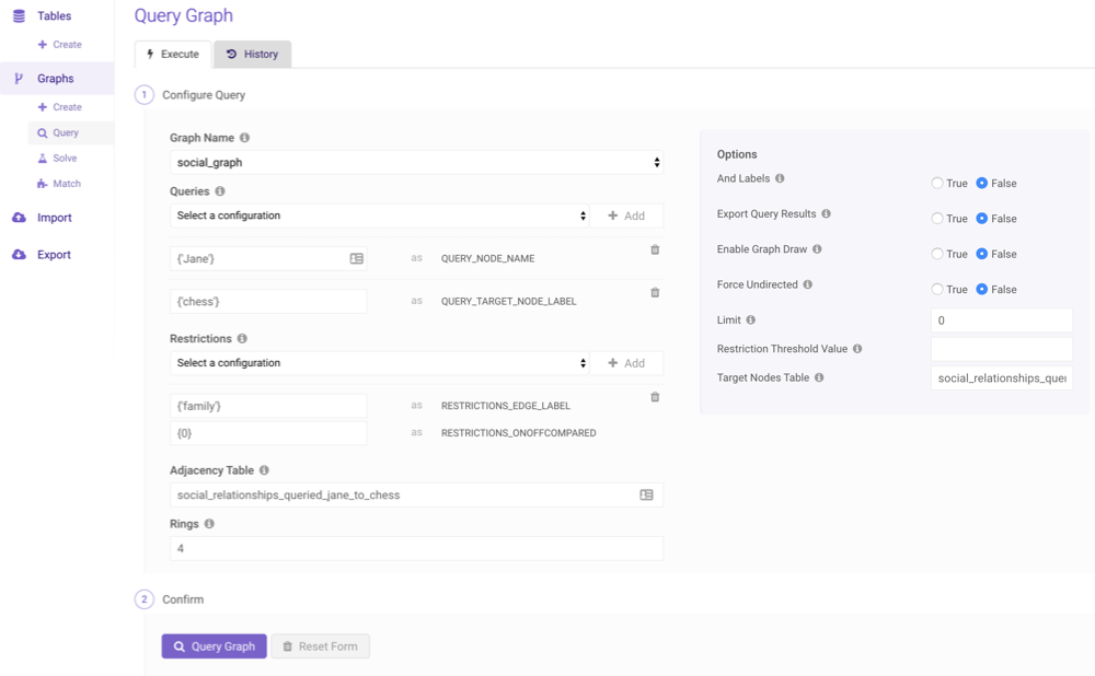
Query
An existing graph can be queried by clicking Query (underneath Graphs) on the left menu to navigate to the Query Graph page. Follow the steps below to query a graph using the interface:
Important
It's highly recommended you consult Querying a Graph and /query/graph for information on query identifiers, valid query configurations, query combinations, and query graph options before querying a graph with GAdmin.
- Select an existing graph from the Graph Name drop-down menu.
- Select a desired query configuration from the Queries drop-down menu and click Add +. For each query identifier that appears after adding the configuration, provide a column name, expression, or raw value (as outlined in Components and Identifiers) to use with the query identifier. Repeat as necessary.
- Optionally, select a desired restriction configuration from the Restrictions drop-down menu and click Add +. For each identifier that appears after adding the configuration, provide a column name, expression, or raw value (as outlined in Components and Identifiers) to use with the identifier. Repeat as necessary.
- Provide an adjacency table name into which the results will be output.
- Provide the number of rings (or hops) for the query.
- Adjust the options as desired.
- Click Query Graph.
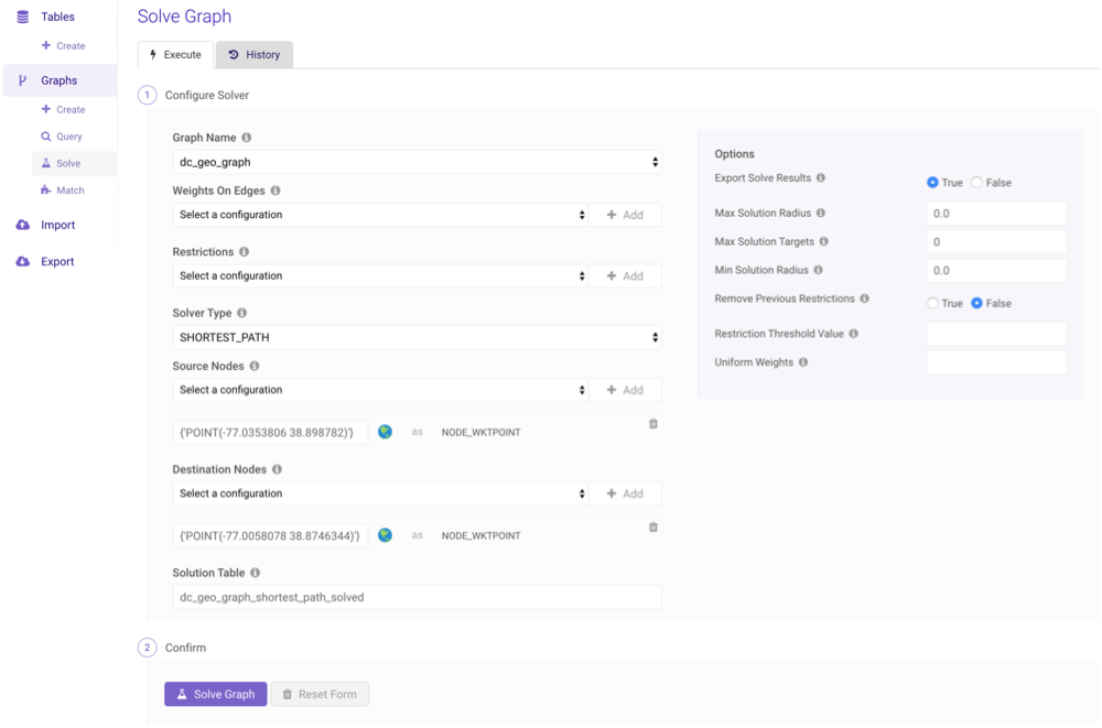
Solve
An existing graph can be solved using a variety of methods by clicking Solve (underneath Graphs) on the left menu to navigate to the Solve Graph page. Follow the steps below to solve a graph using the interface:
Important
It's highly recommended you consult Network Graphs & Solvers Concepts, /solve/graph, and the Solve Graph examples for information on identifiers, valid configurations, combinations, and options before solving a graph with GAdmin.
Select an existing graph from the Graph Name drop-down menu.
Optionally, select a desired weight configuration from the Weights on Edges drop-down menu and click Add +. For each identifier that appears after adding the configuration, provide a column name, expression, or raw value (as outlined in Components and Identifiers) to use with the identifier. Repeat as necessary.
Optionally, select a desired restriction configuration from the Restrictions drop-down menu and click Add +. For each identifier that appears after adding the configuration, provide a column name, expression, or raw value (as outlined in Components and Identifiers) to use with the identifier. Repeat as necessary.
Select a solver from the Solver Type drop-down menu.
Select a node type from the Source Nodes drop-down menu and click Add +. For each field that appears after adding the node type, provide a column name, expression, or raw value (as outlined in Components and Identifiers) to use with the identifier. Repeat as necessary. If adding multiple source nodes, they should all be of the same type.
Tip
If you select
NODE WKTPOINT, you can click to open
the graph in the WMS viewer and manually select point(s) on the map.
to open
the graph in the WMS viewer and manually select point(s) on the map.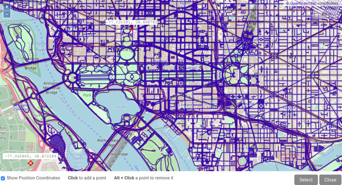
Select a node type from the Destination Nodes drop-down menu and click Add +. For each field that appears after adding the node type, provide a column name, expression, or raw value (as outlined in Components and Identifiers) to use with the identifier. Repeat as necessary. If adding multiple source nodes, they should all be of the same type.
Tip
If you select
NODE WKTPOINT, you can click to open
the graph in the WMS viewer and manually select point(s) on the map.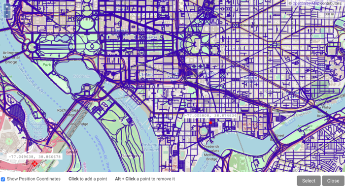
Provide a solution table name into which the results will be output.
Adjust the options as desired.
Click Solve Graph. A WMS request of the solution(s) will open. Click a solution route to see the start (
 ) and end (
 ) points:
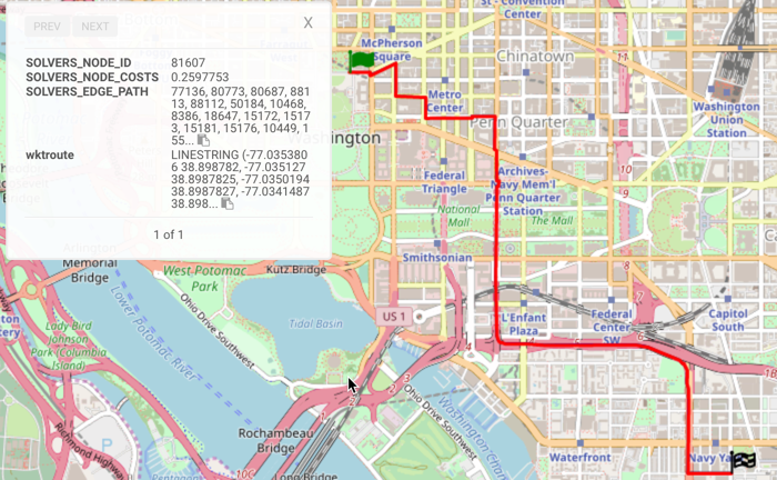
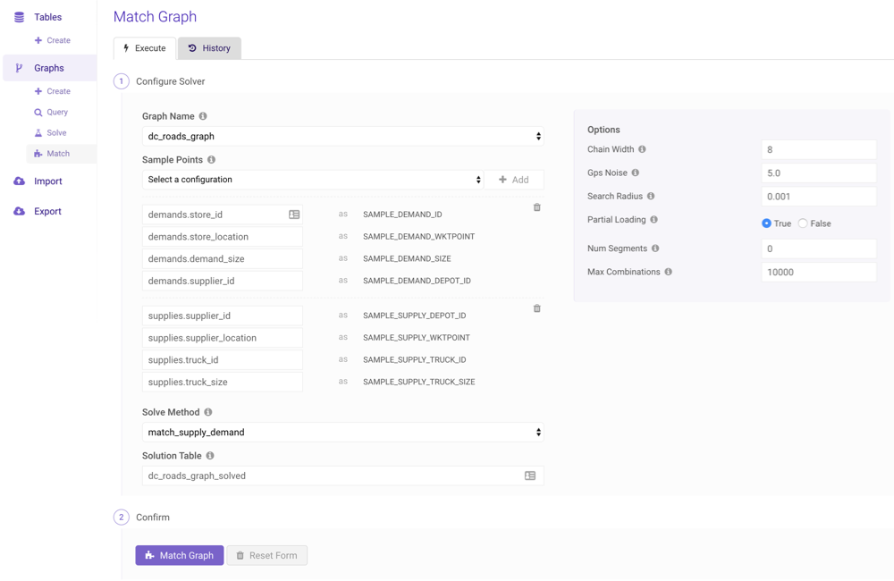
Match
An existing graph can be matched using a variety of methods by clicking Match (underneath Graphs) on the left menu to navigate to the Match Graph page. Follow the steps below to match a graph using the interface:
Important
It's highly recommended you consult Matching a Graph, /match/graph, and the Match Graph examples for information on identifiers, valid configurations, combinations, and options before matching a graph with GAdmin.
- Select an existing graph from the Graph Name drop-down menu.
- Select a sample points configuration from the Sample Points drop-down menu and click Add +. For each field that appears after adding the configuration, provide a column name, expression, or raw value (as outlined in Components and Identifiers) to use with the identifier. Repeat as necessary.
- Select a solver from the Solve Method drop-down menu.
- Provide a solution table name into which the results will be output.
- Adjust the options as desired.
- Click Match Graph.
Import
Data can be imported from many types of files on the Import page. There are three types of import methods available:
- Drag & Drop Import -- default import method
- Advanced Import -- Kinetica Input/Output (KIO) Tool
- Advanced CSV Import -- CSV importing with additional options and control
Drag & Drop Import and Advanced Import jobs have access to the Transfer Status window, which provides detailed information about the transfer:

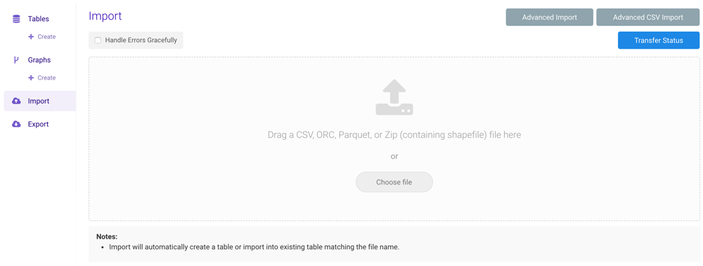
Drag & Drop
Drag & Drop Import currently supports the following file types:
- CSV
- ORC
- Parquet
- Shapefile (as a .zip file)
Drag & Drop Import is the simplest of the three methods: drag a file from a local directory into the drop area of GAdmin, or click Choose file to manually select a local file.
If the file's name matches an existing table's name (and matches the table's schema), the records will appended to the existing table; if the file's name does not match an existing table's name, a new table named after the file will be created and the records will be inserted into it. Geometry columns will be automatically inferred based on the source data. No additional customization is available.
Use the Handle Errors Gracefully check box to have Kinetica gracefully handle errors during import and attempt to finish.
Once the table upload is complete, click View Table to view the imported records:

Advanced Import
Advanced Import currently supports importing from the following sources:
- AWS S3
- CSV
- Parquet
- Parquet Dataset
- Kinetica tables
- Local Storage (files stored on Kinetica's head node)
- CSV
- ORC
- Parquet
- Shapefile
- Oracle
- PostgreSQL / PostGIS
- SQL Server / GIS
- Sybase IQ
- Teradata
Tip
For imports from local storage, files can also be manually uploaded via the Advanced Import interface if Local Storage is selected as the Datasource.
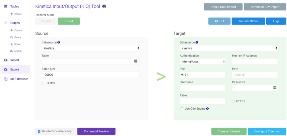
The Advanced Import is the GAdmin version of the Kinetica Input/Output (KIO) Tool. Advanced Import provides the ability to import data from a source to this instance of Kinetica using KIO and Spark. For information on how to interact with KIO from the command line, see KIO. For more on how to export data, see Export.
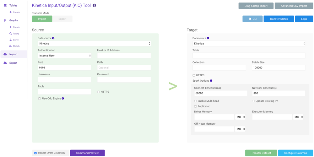
To import data, ensure the Import mode is selected. For the Source section, select a source and fill the required fields. For the Target section, type a name for the table, optionally provide a collection name and update the Spark options, then click Transfer Dataset. If the table exists, the data will be appended to the table; if the table does not exist, it will be created and the data will be inserted into it. The Transfer Status window will automatically open to inform you of the status of the transfer. Click Logs to view the KIO logs at any time. Click Command Preview to see the corresponding KIO CLI command for the configured Source / Target fields.
Use the Handle Errors Gracefully check box to have Kinetica gracefully handle errors during import and attempt to finish.
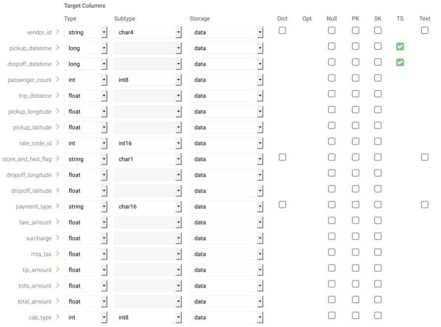
Configure Columns
Once all required fields have been filled, columns from incoming data can be configured before importing into Kinetica. Click Configure Columns to enable column configuration. Kinetica will supply its inferred column configurations, but the type, subtype, storage type, and properties are all user-customizable. See Types for more details on column types, subtypes, storage, and properties.
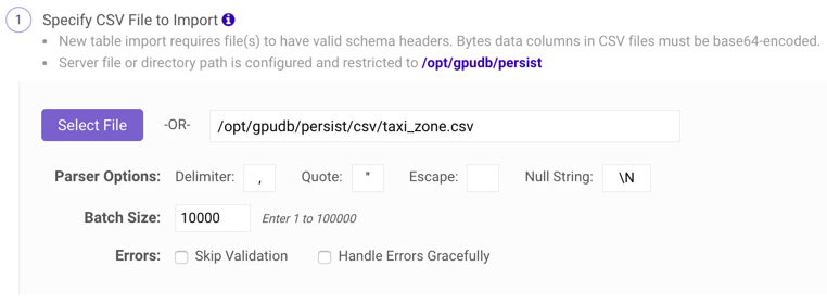
Advanced CSV Import
Advanced CSV Import allows you to customize the way a CSV file is
imported. First upload a file using the Select File button or
providing a directory path. The file in the given directory must be accessible
to the gpudb user and reside on the path (or relative to the path) specified
by the external files directory in the
Kinetica configuration file. Next, type the delimiter (,, |, etc.),
quote character (", ', etc.), escape character (\, ", etc.),
null string value (\N, etc.), whether Kinetica should skip initial file
validation and/or handle errors gracefully (skip over rows with parsing errors),
and the batch size, then choose whether to import the data into a new table or
one that already exists.
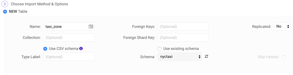
If you want to create a new table, you must at least specify the table name, but you can optionally specify a collection name, a type label (if specifying a type header using the first row of the CSV file as described in Export Data), a foreign key, a foreign shard key, an existing type label (if not creating a new type), and replication.
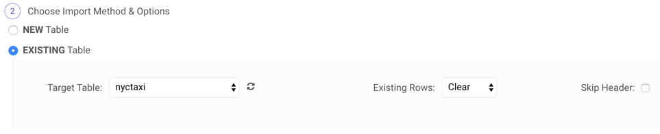
If you want to import data into a table that already exists, you just need to specify the table name, whether to clear any rows that already exist, and whether to skip the header (the first row) present in the file.
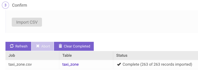
When ready, click Import CSV and the system will provide feedback as it is importing the data.
Export
Export provides the ability to export data from this instance of Kinetica to a target. The following targets are currently supported for exporting:
- AWS S3
- CSV
- Kinetica tables
- Local Storage (files stored on Kinetica's head node)
- CSV
- Parquet
- PostgreSQL
To export data, ensure the Export mode is selected. For the Source section, select a table in Kinetica. For the Target section, select a target and fill the required fields, then click Transfer Dataset. The Transfer Status window will automatically open to inform you of the status of the transfer.
Configure Columns
If exporting to another table in Kinetica, columns from the table being exported can be configured once all required fields have been filled. Click Configure Columns to enable column configuration. Kinetica will supply the columns' current configurations, but the type, subtype, storage type, and properties are all user-customizable. See Types for more details on column types, subtypes, storage, and properties.