This documentation is for a prior release of Kinetica. For the latest documentation, click
here.
Generate Isochrones
Learn how to create isochrones with Kinetica's Graph
The following is a complete example, using the Python API, of generating
images containing isochrones via the /visualize/isochrone
and /wms endpoints using an existing
graph.
Prerequisites
The prerequisites for running the isochrones example are listed below:
Change directory into the newly downloaded repository:
1
cd kinetica-api-python
In the root directory of the unzipped repository, install the Kinetica API:
1
sudo python setup.py install
Test the installation (Python 2.7 (or greater) is necessary for running the
API example):
1
python examples/example.py
Data File
The example script references the dc_shape.csv data file,
mentioned in the Prerequisites, in the current local directory, by default.
This directory can specified as a parameter when running the script.
Script Detail
This example is going to demonstrate the following scenarios using isochrones
either via the /visualize/isochrone endpoint or the
/wms endpoint:
Find the shared area between Dulles International Airport (IAD), Ronald
Reagan Washington National Airport (DCA),and Kinetica HQ by calculating the
isochrones for traveling to IAD within 40 minutes, traveling to
DCA within 25 minutes, and traveling from Kinetica HQ within 10 minutes
and joining the results on the intersection of the isochrones using
/visualize/isochrone
Calculating the isochrones for traveling to Kinetica HQ within 15 minutes
using /wms
Connections
This example will use two connections, one to the database and one to the WMS
endpoint, configured as follows:
SCHEMA -- the name of the schema in which the tables will be created
TABLE_DC -- the name of the table into which the DC Shape dataset is
loaded
TABLE_D_LVL -- the name of the table into which the IAD isochrone
contour levels are output
TABLE_JOIN -- the name of the join view hosting the shared area between
the three isochrone contour level output tables
TABLE_K_ISO_SOLVE -- the name of the table into which the WMS examples'
isochrones solution (the position and cost for each vertex in the underlying
graph) is output
TABLE_K_LVL1 -- the name of the table into which the Kinetica isochrone
(leading from) contour levels are output
TABLE_K_LVL2 -- the name of the table into which the Kinetica isochrone
(leading to) contour levels are output
TABLE_R_LVL -- the name of the table into which the DCA isochrone
contour levels are output
GRAPH_DC -- the underlying DC shape graph that powers the isochrone
calculation
D_AIR, K_HQ, R_AIR -- the source nodes for the IAD, Kinetica HQ, &
DCA isochrone requests,
respectively
D_AIR_IMG, K_HQ_IMG1, K_HQ_IMG2, R_AIR_IMG -- the resulting
generated isochrone image from the IAD, Kinetica HQ (leading from),
Kinetica HQ (leading to), & DCA isochrone requests, respectively
Graph Creation
One graph is used for the isochrones examples utilized in the script:
dc_shape_graph, a graph based on the dc_shape dataset (the CSV file
mentioned in Prerequisites).
Note
The example script will first check to see if the dc_shape table
and dc_shape_graph exist; if either does not, they will be
created.
The dc_shape_graph is created with the following characteristics:
It is directed because the roads in the graph have
directionality (one-way and two-way roads)
It has no explicitly defined nodes because the nodes are not used in these
examples
The edges are represented using WKT LINESTRINGs in the shape column
of the dc_shape table (WKTLINE). Each edge's directionality is
derived from the direction column of the dc_shape
table (DIRECTION).
The weights represent the time taken to travel the edge, which
is derived from the length of the edge divided by the speed column values
also found in the dc_shape table. This derived time value is mapped to the
VALUESPECIFIEDidentifier.
It has no inherent restrictions for any of the nodes or edges in the graph
It will be replaced with this instance of the graph if a graph of the same
name exists (recreate)
Create Graph
 1
 2
 3
 4
 5
 6
 7
 8
 9
10
11
12
13
14
15
16
create_graph_dc_resp=kinetica.create_graph(graph_name=GRAPH_DC,directed_graph=True,nodes=[],edges=[TABLE_DC+".direction AS DIRECTION",TABLE_DC+".shape AS WKTLINE"],weights=[TABLE_DC+".direction AS EDGE_DIRECTION",TABLE_DC+".shape AS EDGE_WKTLINE","ST_LENGTH("+TABLE_DC+".shape,1)/"+TABLE_DC+".speed AS VALUESPECIFIED"],restrictions=[],options={"recreate":"true"})
The graph output to WMS:
Visualizing Isochrones
First, additional contour and isochrones options are provided:
add_labels is set to true to display labels on the isochrones image
projection is set to web_mercator to change the spatial reference
system
solve_direction is set to to_source to calculate isochrones leading
to IAD
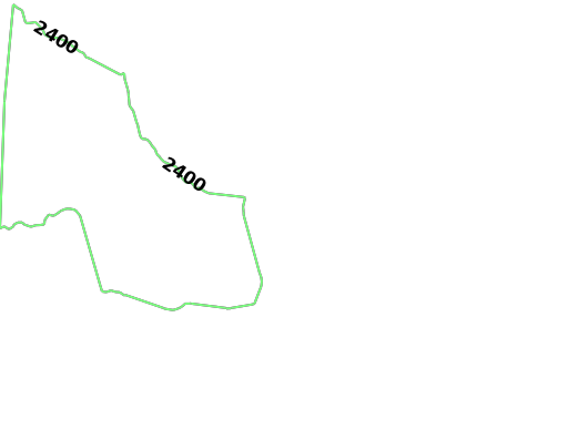
Then, the first group of isochrones is calculated using the following
parameters and an image is generated using
/visualize/isochrone endpoint:
source_node is provided as a WKT point (D_AIR) paired with a
NODE_WKTPOINTidentifier
max_solution_radius is set for 2400 seconds' (or 40 minutes') worth of
travel surrounding the source node
num_levels is set to 1 to only display one isochrone contour around
the source node
generate_image is set to True to generate an image and output it to
the response
Request IAD Isochrone Image
1
2
3
4
5
6
7
8
9
10
11
vis_isochrone_d_resp=kinetica.visualize_isochrone(graph_name=GRAPH_DC,source_node=D_AIR+" AS NODE_WKTPOINT",max_solution_radius=40*60,num_levels=1,generate_image=True,levels_table=TABLE_D_LVL,style_options=OPTION_ISO_STYLE,contour_options=OPTION_ISO_CONTOUR,options=OPTION_ISO)
The image is pulled from the response and written locally:
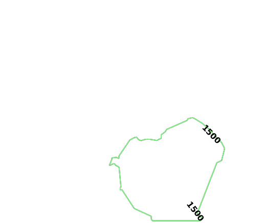
The second group of isochrones is calculated using the following parameters:
Note
The solve_direction is still to_source at this point, so
the second group of isochrones is calculated for leading to
DCA
source_node is provided as a WKT point (R_AIR) paired with a
NODE_WKTPOINTidentifier
max_solution_radius is set for 1500 seconds' (or 25 minutes') worth of
travel surrounding the source node
num_levels is set to 1 to only display one isochrone contour around
the source node
generate_image is set to True to generate an image and output it to
the response
Request DCA Isochrone Image
1
2
3
4
5
6
7
8
9
10
11
vis_isochrone_r_resp=kinetica.visualize_isochrone(graph_name=GRAPH_DC,source_node=R_AIR+" AS NODE_WKTPOINT",max_solution_radius=25*60,num_levels=1,generate_image=True,levels_table=TABLE_R_LVL,style_options=OPTION_ISO_STYLE,contour_options=OPTION_ISO_CONTOUR,options=OPTION_ISO)
The image is pulled from the response and written locally:
Before the last example, the solve direction is updated to reflect that the
isochrones are calculated leading from Kinetica HQ:
Update Solve Orientation
1
OPTION_ISO["solve_direction"]="from_source"
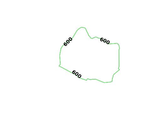
Finally, the third group of isochrones can be calculated using the following
parameters:
source_node is provided as a WKT point (K_HQ) paired with a
NODE_WKTPOINTidentifier
max_solution_radius is set for 600 seconds' (or 10 minutes') worth of
travel surrounding the source node
num_levels is set to 1 to only display one isochrone contour around
the source node
generate_image is set to True to generate an image and output it to
the response
Request Kinetica HQ Isochrone Image
 1
 2
 3
 4
 5
 6
 7
 8
 9
10
11
vis_isochrone_k1_resp=kinetica.visualize_isochrone(graph_name=GRAPH_DC,source_node=K_HQ+" AS NODE_WKTPOINT",max_solution_radius=10*60,num_levels=1,generate_image=True,levels_table=TABLE_K_LVL1,style_options=OPTION_ISO_STYLE,contour_options=OPTION_ISO_CONTOUR,options=OPTION_ISO)
The image is pulled from the response and written locally:
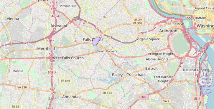
The generated image for Kinetica HQ (leading from) isochrones:
To find the shared area between the three contours that were just created,
the ST_INTERSECTION() geospatial function is used to join the three tables
together:
Geospatial Intersection via Join
1
2
3
4
5
6
7
8
9
10
11
12
13
create_join_resp=kinetica.create_join_table(join_table_name=TABLE_JOIN,table_names=[TABLE_D_LVL+" AS DULLES",TABLE_K_LVL1+" AS KINETICA",TABLE_R_LVL+" AS REAGAN"],column_names=["ST_INTERSECTION(REAGAN.Isochrones, ST_INTERSECTION(KINETICA.Isochrones, DULLES.Isochrones)) AS shared_isochrones"],expressions=[],options={})
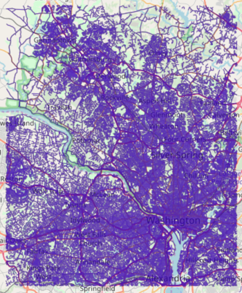
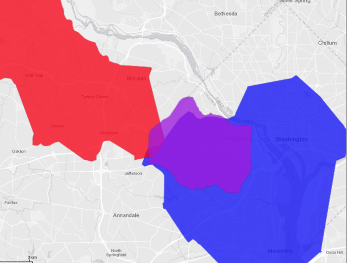
The shared area geometry output to WMS:
The three isochrones overlaid on top of each other:
Red signifies being within 40 minutes of IAD
Blue signifies being within 25 minutes of DCA
Purple signifies being within 10 minutes of Kinetica HQ
Visualizing Isochrones Using WMS
To visualize isochrones via the /wms endpoint, the WMS
payload must be constructed. Consult /wms for more
information on WMS parameters, styles, and style options.
WMS payloads require a small set of standard parameters that will generally be
the same across all WMS requests:
The next settings inform WMS to generate isochrones (and to make Isochrones
parameters available for use) and to set the image width to 512 pixels. The
image height is set to -1, which the database will replace with the value
resulting from multiplying the aspect ratio by the image width.
The following parameters define how the isochrones will be calculated. Notice
these are similar to the previous examples:
source_node is provided as a WKT point (K_HQ) paired with a
NODE_WKTPOINTidentifier
max_solution_radius is set for 900 seconds' (or 15 minutes') worth of
travel surrounding the source node
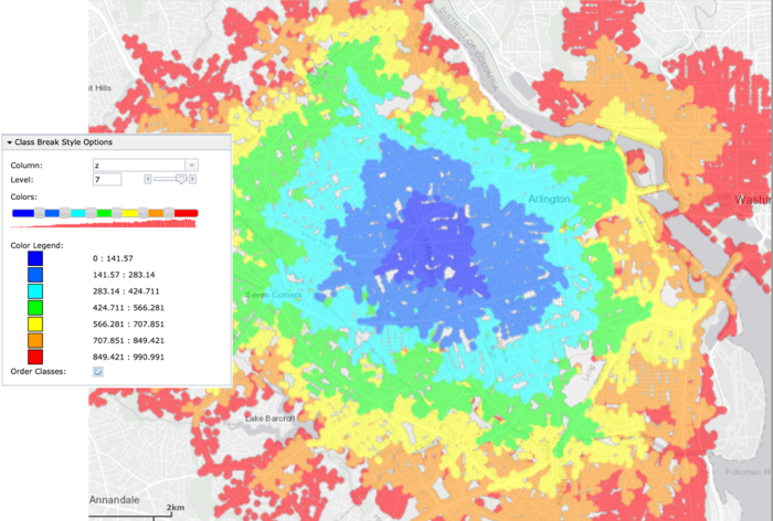
num_levels is set to 10 to 10 isochrone contours around
the source node
generate_image is set to True to generate an image and output it to
the response
Kinetica HQ Isochrone Parameters
1
2
3
4
5
6
"graph_name":GRAPH_DC,"source_node":K_HQ+" AS NODE_WKTPOINT","max_solution_radius":"900","num_levels":"10","generate_image":"true","levels_table":TABLE_K_LVL2,
Isochrone style options are passed in using the constants:
Isochrone Style Parameters
1
2
3
4
"line_size":OPTION_ISO_STYLE["line_size"],"color":OPTION_ISO_STYLE["color"][2:],# remove the 0x"bg_color":OPTION_ISO_STYLE["bg_color"][2:],# remove the 0x"colormap":OPTION_ISO_STYLE["colormap"],
Isochrone contour options are passed in. Additional contour style parameters
are passed in for additional customization over the generated isochrones:
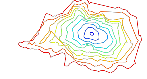
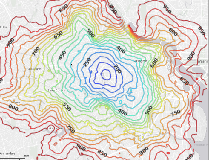
Lastly, isochrone options are passed in. Note the change in direction for the
solve_direction as we want isochrones leading to Kinetica HQ in this
instance.