Shortest Path with Turn Penalties & Restrictions

Python API Installation

The native Kinetica Python API is accessible through the following means:

• PyPI
• Git

Data File

The example script references the dc_shape.csv data file, mentioned in the Prerequisites, in the current local directory, by default. This directory can specified as a parameter when running the script.

The dc_shape dataset is a HERE dataset and is analogous to most road network datasets you could find in that it includes columns for the type of road, the average speed, the direction of the road, a WKT linestring for its geographic location, a unique ID integer for the road, and more. The graph used in the example is created with four columns from the dc_shape dataset:

• link_id -- a sharded integer column composed of unique IDs for each road segment mapped within this dataset
• shape -- a WKT linestring composed of points that make up various streets, roads, highways, alleyways, and footpaths throughout Washington, D.C.; this column is also part of an inline calculation for distance as weight during graph creation
• direction -- an integer column that conveys information about the directionality of the road, with forward meaning the direction in which the way is drawn in OSM and backward being the opposite direction:
  • 0 -- a forward one-way road
  • 1 -- a two-way road
  • 2 -- a backward one-way road
• speed -- an integer column that represents the average speed traveled on a given road segment; this column is also part of an inline calculation for distance as weight during graph creation

Constants

Several constants are defined at the beginning of the script:

• SCHEMA -- the name of the schema in which the tables supporting the graph creation and solve operations will be created

  Important

  The schema is created during the table setup portion of the script because the schema must exist prior to creating the tables that will later support the graph creation and match operations.

• TABLE_DC -- the name of the table into which the D.C. road network dataset is loaded

• GRAPH_DC -- the D.C. road network graph

• SOLUTION_GRAPH_DC_1 / SOLUTION_GRAPH_DC_1 / SOLUTION_GRAPH_DC_3 -- the D.C. road network graph shortest path solution tables

1
2
3
4
5
6
7

SCHEMA = "graph_s_dc_shortest_path_turn"
TABLE_DC = SCHEMA + ".dc_shape"

GRAPH_DC = SCHEMA + ".dc_shape_graph"
SOLUTION_GRAPH_DC_1 = GRAPH_DC + "_solved_sp"
SOLUTION_GRAPH_DC_2 = GRAPH_DC + "_solved_sp_intersection-penalty"
SOLUTION_GRAPH_DC_3 = GRAPH_DC + "_solved_sp_turn-restriction"

Table Setup

Before the graph can be created, the D.C. shape dataset is loaded from a local CSV file. First, the D.C. shape table is created using the GPUdbTable interface:

 1
 2
 3
 4
 5
 6
 7
 8
 9
10
11
12
13

table_dc_obj = gpudb.GPUdbTable(
    _type = [
        ["link_id", "long", "shard_key"],
        ["direction", "int"],
        ["speed", "double"],
        ["road_type", "string", "char1"],
        ["seg", "string", "wkt"],
        ["shape", "string", "wkt"],
    ],
    name = TABLE_DC,
    db = kinetica,
    options = {}
)

Then, the CSV file is uploaded into KiFS and loaded into the table:

1
2
3

kinetica.create_directory("data", {"no_error_if_exists":"true"});
kinetica.upload_files("/data/" + CSV_FILE, open(csv_path, "rb").read())
kinetica.insert_records_from_files(TABLE_DC, ["kifs://data/" + CSV_FILE])

Graph Creation

One graph is used for the shortest path solve graph example utilized in the script: GRAPH_DC, a graph based on the dc_shape dataset (the CSV file mentioned in Prerequisites).

The GRAPH_DC graph is created with the following characteristics:

• It is directed because the roads in the graph have directionality (one-way and two-way roads)
• It has no explicitly defined nodes because the example relies on implicit nodes attached to the defined edges
• The edges are identified by WKTLINE, using from WKT LINESTRINGs from the shape column of the dc_shape table. Each road segment's directionality (DIRECTION) is derived from the direction column of the dc_shape table. Each edge is associated with an ID from the link_id column. Rather than separately define weights, each edge has its weight (WEIGHT_VALUESPECIFIED) calculated inline as the length of the entire shape column's LINESTRING (in meters) divided by the number of points in the LINESTRING minus 1 divided by the average speed used to traverse the LINESTRING.
• It has no inherent restrictions for any of the edges in the graph
• It utilizes the following options:
  • It will be replaced with this instance of the graph if a graph of the same name exists (recreate)
  • The graph will register dummy edges around each intersection of edges generated from the data to represent turns (add_turns)

 1
 2
 3
 4
 5
 6
 7
 8
 9
10
11
12
13
14
15
16
17
18
19

cg = kinetica.create_graph(
    graph_name = GRAPH_DC,
    directed_graph = True,
    nodes = [],
    edges = [
        TABLE_DC + ".link_id AS ID",
        TABLE_DC + ".shape AS WKTLINE",
        TABLE_DC + ".direction AS DIRECTION",
        "(ST_LENGTH(" + TABLE_DC + ".shape,1)/"
        "(ST_NPOINTS(" + TABLE_DC + ".shape)-1))/" + 
        TABLE_DC + ".speed AS WEIGHT_VALUESPECIFIED"
    ],
    weights = [],
    restrictions = [],
    options = {
        "recreate": "true",
        "add_turns": "true"
    }
)

Shortest Path

No Turn Penalties or Restrictions

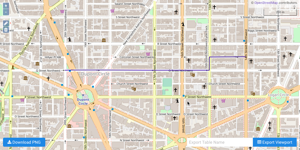
The first example illustrates a simple shortest path solve from a single source node to a single destination node. First, the source node and destination node are defined.

Note

The source and destination node are the same for each example.

Define Beginning & Ending Points

1 2	src = ["POINT(-77.04489135742188 38.91112899780273)"] dest = ["POINT(-77.03193664550781 38.91188049316406)"]

Next, the GRAPH_DC graph is solved with the solve results being exported to the response:

Solve Graph for Shortest Path without Penalties or Restrictions

1 2 3 4 5 6 7

kinetica.solve_graph( graph_name = GRAPH_DC, solver_type = "SHORTEST_PATH", source_nodes = src, destination_nodes = dest, solution_table = SOLUTION_GRAPH_DC_1 )

The cost for the source node to visit the destination node is represented as time in seconds:

Solve Graph for Shortest Path without Penalties or Restrictions Solution

1 2 3 4 5

+---------------------+ | Cost (in seconds) | |---------------------| | 106.994 | +---------------------+

The solution output to WMS:

Intersection Penalty

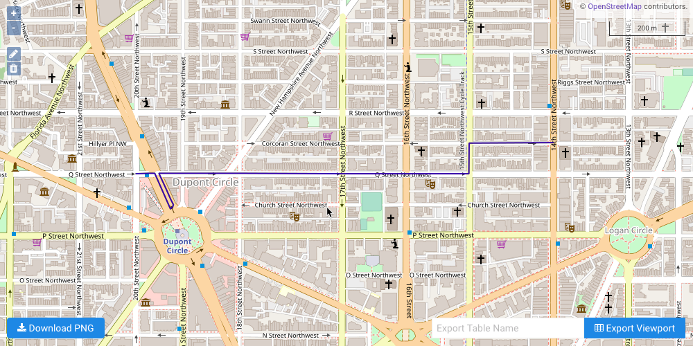
The second example illustrates a shortest path solve from a single source node to a single destination node, but this time traveling through an intersection of two-way roads will incur an additional cost. The GRAPH_DC graph is solved with the solve results being exported to the response and an intersection penalty of 20 seconds:

Solve Graph for Shortest Path with Intersection Penalties

1 2 3 4 5 6 7 8 9 10

kinetica.solve_graph( graph_name = GRAPH_DC, solver_type = "SHORTEST_PATH", source_nodes = src, destination_nodes = dest, solution_table = SOLUTION_GRAPH_DC_2, options = { "intersection_penalty": "20" } )

The cost for the source node to visit the destination node is represented as time in seconds:

Solve Graph for Shortest Path with Intersection Penalties Solution

1 2 3 4 5

+---------------------+ | Cost (in seconds) | |---------------------| | 155.317 | +---------------------+

The solution output to WMS, noting the immediate U-turn to return to Q Street from Connecticut Avenue to avoid the intersection penalty:

Turn Restriction

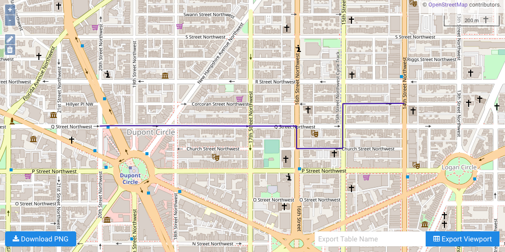
The third example illustrates a shortest path solve from a single source node to a single destination node, but this time a single turn from Q Street on to 15th Street is restricted. The GRAPH_DC graph is solved with turns from road segment ID 18352169 (Q Street) to road segment ID 18352166 (15th Street) being restricted and the solve results being exported to the response:

Solve Graph for Shortest Path with Turn Restrictions

1 2 3 4 5 6 7 8 9 10 11 12

kinetica.solve_graph( graph_name = GRAPH_DC, restrictions = [ "{18352169} AS FROM_EDGE_ID", "{18352166} AS TO_EDGE_ID", "{0} AS ONOFFCOMPARED" ], solver_type = "SHORTEST_PATH", source_nodes = src, destination_nodes = dest, solution_table = SOLUTION_GRAPH_DC_3 )

The cost for the source node to visit the destination node is represented as time in seconds:

Solve Graph for Shortest Path with Turn Restrictions Solution

1 2 3 4 5

+---------------------+ | Cost (in seconds) | |---------------------| | 108.284 | +---------------------+

The solution output to WMS, noting the detour on to 16th Street and Church Street to avoid the restricted turn: