Isochrones

The following is a complete example, using the Python API, of generating images containing isochrones via the /visualize/isochrone and /wms endpoints using an existing graph.

Prerequisites

The prerequisites for running the isochrones example are listed below:

• Kinetica (v. 7.0.4 or later)
• Graph server enabled
• Python API
• Isochrones example script
• DC Shape data CSV file

Python API Installation

The native Kinetica Python API is accessible through the following means:

• For development on the Kinetica server:
  • Kinetica RPM
• For development not on the Kinetica server:
  • Git
  • PyPI

Kinetica RPM

In default Kinetica installations, the native Python API is located in the /opt/gpudb/api/python directory. The /opt/gpudb/bin/gpudb_python wrapper script is provided, which sets the execution environment appropriately.

Test the installation:

/opt/gpudb/bin/gpudb_python /opt/gpudb/api/python/examples/example.py

Important

When developing on the Kinetica server, use /opt/gpudb/bin/gpudb_python to run Python programs and /opt/gpudb/bin/gpudb_pip to install dependent libraries.

Git

1. In the desired directory, run the following but be sure to replace <kinetica-version> with the name of the installed Kinetica version, e.g., v7.0:

   git clone -b release/<kinetica-version> --single-branch https://github.com/kineticadb/kinetica-api-python.git
   

2. Change directory into the newly downloaded repository:

   cd kinetica-api-python
   

3. In the root directory of the unzipped repository, install the Kinetica API:

   sudo python setup.py install
   

4. Test the installation (Python 2.7 (or greater) is necessary for running the API example):

   python examples/example.py
   

PyPI

The Python package manager, pip, is required to install the API from PyPI.

1. Install the API:

   pip install gpudb --upgrade
   

2. Test the installation:

   python -c "import gpudb;print('Import Successful')"
   

   If Import Successful is displayed, the API has been installed as is ready for use.

Data Files

The example script makes reference to a dc_shape.csv data file in the current directory. This can be updated to point to a valid path on the host where the file will be located, or the script can be run with the data file in the current directory.

CSV = "dc_shape.csv"

Script Detail

This example is going to demonstrate the following scenarios using isochrones either via the /visualize/isochrone endpoint or the /wms endpoint:

• Find the shared area between Dulles International Airport (IAD), Ronald Reagan Washington National Airport (DCA),and Kinetica HQ by calculating the isochrones for traveling to IAD within 40 minutes, traveling to DCA within 25 minutes, and traveling from Kinetica HQ within 10 minutes and joining the results on the intersection of the isochrones using /visualize/isochrone
• Calculating the isochrones for traveling to Kinetica HQ within 15 minutes using /wms

Constants

Many constants are defined at the beginning of the script:

• CSV_ROW_SIZE -- the expected row number for the CSV file
• DB_HOST / DB_PORT -- host and port values for the database
• WMS_URL -- the URL string for the /wms endpoint

CSV_ROW_SIZE = 192238
DB_HOST = "127.0.0.1"
DB_PORT = "9191"
WMS_URL = "http://" + DB_HOST + ":" + DB_PORT + "/wms"

• OPTION_NO_ERROR -- reference to a /clear/table option for ease of use and repeatability
• OPTION_ISO -- a Python dictionary containing /visualize/isochrone options key-value pairs
• OPTION_ISO_CONTOUR -- a Python dictionary containing /visualize/isochrone contour_options key-value pairs
• OPTIONS_ISO_STYLE -- a Python dictionary containing /visualize/isochrone style_options key-value pairs

OPTION_NO_ERROR = {"no_error_if_not_exists": "true"}
OPTION_ISO = {"concavity_level": "0.2", "is_replicated": "true"}
OPTION_ISO_CONTOUR = {
    "adjust_grid": "false",
    "adjust_levels": "false",
    "gridding_method": "INV_DST_POW",
    "labels_font_size": "16",
    "labels_font_family": "Sans",
    "labels_search_window": "4",
    "grid_size": str(100),
    "min_grid_size": "10",
    "max_grid_size": "300",
    "search_radius": "9",
    "smoothing_factor": "0.000001",
    "color_isolines": "true",
    "width": "512", "height": "-1"
}
OPTION_ISO_STYLE = {
    "line_size": "2",
    "color": "0xFF000000",
    "bg_color": "0x00000000",
    "colormap": "jet",
    "text_color": "0xFF000000"
}

• TABLE_DC -- the name of the table into which the DC Shape dataset is loaded
• TABLE_D_LVL -- the name of the table into which the IAD isochrone contour levels are output
• TABLE_JOIN -- the name of the join view hosting the shared area between the three isochrone contour level output tables
• TABLE_K_ISO_SOLVE -- the name of the table into which the WMS examples' isochrones solution (the position and cost for each vertex in the underlying graph) is output
• TABLE_K_LVL1 -- the name of the table into which the Kinetica isochrone (leading from) contour levels are output
• TABLE_K_LVL2 -- the name of the table into which the Kinetica isochrone (leading to) contour levels are output
• TABLE_R_LVL -- the name of the table into which the DCA isochrone contour levels are output

TABLE_DC = "dc_shape"
TABLE_D_LVL = "dulles_levels"
TABLE_JOIN = "isochrones_shared_area"
TABLE_K_ISO_SOLVE = "to_kinetica_isochrones_solution"
TABLE_K_LVL1 = "from_kinetica_levels"
TABLE_K_LVL2 = "to_kinetica_levels"
TABLE_R_LVL = "reagan_levels"

• GRAPH_DC -- the underlying DC shape graph that powers the isochrone calculation

GRAPH_DC = TABLE_DC + "_graph"

• D_AIR -- the source node for the IAD isochrone request
• K_HQ -- the source node for the Kinetica HQ isochrone requests
• R_AIR -- the source node for the DCA isochrone request

D_AIR = "POINT(-77.446831 38.955309)"
K_HQ = "POINT(-77.115203 38.881578)"
R_AIR = "POINT(-77.042295 38.849684)"

• D_AIR_IMG -- the resulting generated isochrone image from the IAD isochrone request
• K_HQ_IMG1 -- the resulting generated isochrone image from the Kinetica HQ isochrone request (leading from)
• K_HQ_IMG2 -- the resulting generated isochrone image from the Kinetica HQ isochrone request (leading to)
• R_AIR_IMG -- the resulting generated isochrone image from the DCA isochrone request

D_AIR_IMG = TABLE_D_LVL + ".png"
K_HQ_IMG1 = TABLE_K_LVL1 + ".png"
K_HQ_IMG2 = TABLE_K_LVL2 + ".png"
R_AIR_IMG = TABLE_R_LVL + ".png"

Graph Creation

One graph is used for the isochrones examples utilized in the script: dc_shape_graph, a graph based on the dc_shape dataset (the CSV file mentioned in Prerequisites).

Note

The example script will first check to see if the dc_shape table and dc_shape_graph exist; if either does not, they will be created.

The dc_shape_graph is created with the following characteristics:

• It is directed because the roads in the graph have directionality (one-way and two-way roads)
• It has no explicitly defined nodes because the nodes are not used in these examples
• The edges are represented using WKT LINESTRINGs in the shape column of the dc_shape table (EDGE_WKTLINE). Each edge's directionality is derived from the direction column of the dc_shape table (EDGE_DIRECTION).
• The weights represent the time taken to travel the edge, which is derived from the length of the edge divided by the speed column values also found in the dc_shape table. This derived time value is mapped to the WEIGHTS_VALUESPECIFIED identifier.
• It has no inherent restrictions for any of the nodes or edges in the graph
• It will be replaced with this instance of the graph if a graph of the same name exists (recreate)

create_graph_dc_resp = kinetica.create_graph(
    graph_name=GRAPH_DC,
    directed_graph=True,
    nodes=[],
    edges=[
        TABLE_DC + ".direction AS EDGE_DIRECTION",
        TABLE_DC + ".shape AS EDGE_WKTLINE"
    ],
    weights=[
        TABLE_DC + ".direction AS WEIGHTS_EDGE_DIRECTION",
        TABLE_DC + ".shape AS WEIGHTS_EDGE_WKTLINE",
        "ST_LENGTH(" + TABLE_DC + ".shape,1)/" + TABLE_DC + ".speed AS WEIGHTS_VALUESPECIFIED"
    ],
    restrictions=[],
    options={"recreate": "true"}
)

The graph output to WMS:

Visualizing Isochrones

First, additional contour and isochrones options are provided:

• add_labels is set to true to display labels on the isochrones image
• projection is set to web_mercator to change the spatial reference system
• solve_direction is set to to_source to calculate isochrones leading to IAD

OPTION_ISO_CONTOUR["add_labels"] = "true"
OPTION_ISO_CONTOUR["projection"] = "web_mercator"
OPTION_ISO["solve_direction"] = "to_source"

Then, the first group of isochrones is calculated using the following parameters and an image is generated using /visualize/isochrone endpoint:

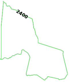
• source_node is provided as a WKT point (D_AIR) paired with a NODE_WKTPOINT identifier
• max_solution_radius is set for 2400 seconds' (or 40 minutes') worth of travel surrounding the source node
• num_levels is set to 1 to only display one isochrone contour around the source node
• generate_image is set to True to generate an image and output it to the response

vis_isochrone_d_resp = kinetica.visualize_isochrone(
    graph_name=GRAPH_DC,
    source_node=D_AIR + " AS NODE_WKTPOINT",
    max_solution_radius=40*60,
    num_levels=1,
    generate_image=True,
    levels_table=TABLE_D_LVL,
    style_options=OPTION_ISO_STYLE,
    contour_options=OPTION_ISO_CONTOUR,
    options=OPTION_ISO
)

The image is pulled from the response and written locally:

img = vis_isochrone_d_resp["image_data"]
img_isochrones_to_dulles = open(D_AIR_IMG, "wb")
img_isochrones_to_dulles.write(img)
img_isochrones_to_dulles.close()

The generated image for IAD isochrones:

The second group of isochrones is calculated using the following parameters:

Note

The solve_direction is still to_source at this point, so the second group of isochrones is calculated for leading to DCA

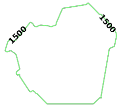
• source_node is provided as a WKT point (R_AIR) paired with a NODE_WKTPOINT identifier
• max_solution_radius is set for 1500 seconds' (or 25 minutes') worth of travel surrounding the source node
• num_levels is set to 1 to only display one isochrone contour around the source node
• generate_image is set to True to generate an image and output it to the response

vis_isochrone_r_resp = kinetica.visualize_isochrone(
    graph_name=GRAPH_DC,
    source_node=R_AIR + " AS NODE_WKTPOINT",
    max_solution_radius=25*60,
    num_levels=1,
    generate_image=True,
    levels_table=TABLE_R_LVL,
    style_options=OPTION_ISO_STYLE,
    contour_options=OPTION_ISO_CONTOUR,
    options=OPTION_ISO
)

The image is pulled from the response and written locally:

img = vis_isochrone_r_resp["image_data"]
img_isochrones_to_reagan = open(R_AIR_IMG, "wb")
img_isochrones_to_reagan.write(img)
img_isochrones_to_reagan.close()
print("Generated PNG file: {}\n".format(R_AIR_IMG))

The generated image for DCA isochrones:

Before the last example, the solve direction is updated to reflect that the isochrones are calculated leading from Kinetica HQ:

OPTION_ISO["solve_direction"] = "from_source"

Finally, the third group of isochrones can be calculated using the following parameters:

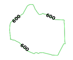
• source_node is provided as a WKT point (K_HQ) paired with a NODE_WKTPOINT identifier
• max_solution_radius is set for 600 seconds' (or 10 minutes') worth of travel surrounding the source node
• num_levels is set to 1 to only display one isochrone contour around the source node
• generate_image is set to True to generate an image and output it to the response

vis_isochrone_k1_resp = kinetica.visualize_isochrone(
    graph_name=GRAPH_DC,
    source_node=K_HQ + " AS NODE_WKTPOINT",
    max_solution_radius=10*60,
    num_levels=1,
    generate_image=True,
    levels_table=TABLE_K_LVL1,
    style_options=OPTION_ISO_STYLE,
    contour_options=OPTION_ISO_CONTOUR,
    options=OPTION_ISO
)

The image is pulled from the response and written locally:

img = vis_isochrone_k1_resp["image_data"]
img_isochrones_from_kinetica = open(K_HQ_IMG1, "wb")
img_isochrones_from_kinetica.write(img)
img_isochrones_from_kinetica.close()

The generated image for Kinetica HQ (leading from) isochrones:

To find the shared area between the three contours that were just created, the ST_INTERSECTION() geospatial function is used to join the three tables together:

create_join_resp = kinetica.create_join_table(
    join_table_name=TABLE_JOIN,
    table_names=[
        TABLE_D_LVL + " AS DULLES",
        TABLE_K_LVL1 + " AS KINETICA",
        TABLE_R_LVL + " AS REAGAN"
    ],
    column_names=[
        "ST_INTERSECTION(REAGAN.Isochrones, ST_INTERSECTION(KINETICA.Isochrones, DULLES.Isochrones)) AS shared_isochrones"
    ],
    expressions=[],
    options={}
)

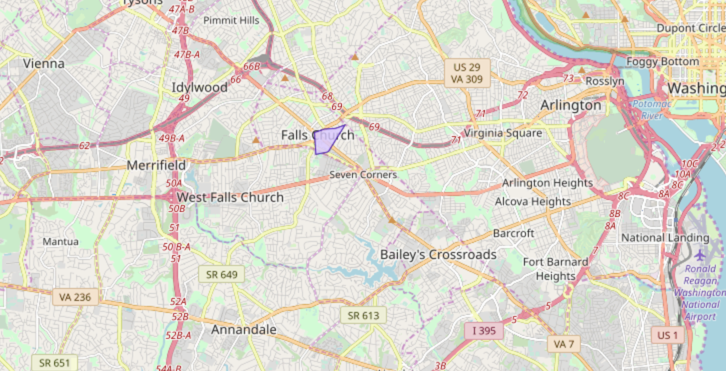
The shared area geometry output to WMS:

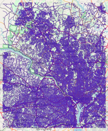
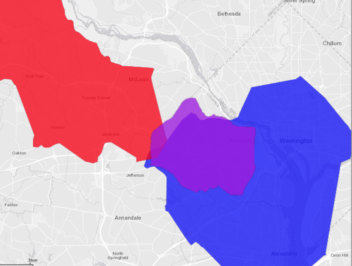
The three isochrones overlaid on top of each other:

• Red signifies being within 40 minutes of IAD
• Blue signifies being within 25 minutes of DCA
• Purple signifies being within 10 minutes of Kinetica HQ

Visualizing Isochrones Using WMS

To visualize isochrones via the /wms endpoint, the WMS payload must be constructed. Consult /wms for more information on WMS parameters, styles, and style options.

WMS payloads require a small set of standard parameters that will generally be the same across all WMS requests:

"request": "GetMap",
"version": "1.1.1",
"format": "image/png",

The next settings inform WMS to generate isochrones (and to make Isochrones parameters available for use) and to set the image width to 512 pixels. The image height is set to -1, which the database will replace with the value resulting from multiplying the aspect ratio by the image width.

"styles": "isochrone",
"image_width": 512,
"image_height": -1,

The following parameters define how the isochrones will be calculated. Notice these are similar to the previous examples:

• source_node is provided as a WKT point (K_HQ) paired with a NODE_WKTPOINT identifier
• max_solution_radius is set for 900 seconds' (or 15 minutes') worth of travel surrounding the source node
• num_levels is set to 10 to 10 isochrone contours around the source node
• generate_image is set to True to generate an image and output it to the response

"graph_name": GRAPH_DC,
"source_node": K_HQ + " AS NODE_WKTPOINT",
"max_solution_radius": "900",
"num_levels": "10",
"generate_image": "true",
"levels_table": TABLE_K_LVL2,

Isochrone style options are passed in using the constants:

"line_size": OPTION_ISO_STYLE["line_size"],
"color": OPTION_ISO_STYLE["color"][2:],  # remove the 0x
"bg_color": OPTION_ISO_STYLE["bg_color"][2:],  # remove the 0x
"colormap": OPTION_ISO_STYLE["colormap"],

Isochrone contour options are passed in. Additional contour style parameters are passed in for additional customization over the generated isochrones:

"projection": "plate_carree",
"search_radius": OPTION_ISO_CONTOUR["search_radius"],
"color_isolines": OPTION_ISO_CONTOUR["color_isolines"],
"add_labels": "false",

"gridding_method": OPTION_ISO_CONTOUR["gridding_method"],
"smoothing_factor": OPTION_ISO_CONTOUR["smoothing_factor"],
"max_search_cells": "100",
"min_grid_size": OPTION_ISO_CONTOUR["min_grid_size"],
"max_grid_size": OPTION_ISO_CONTOUR["max_grid_size"],

Lastly, isochrone options are passed in. Note the change in direction for the solve_direction as we want isochrones leading to Kinetica HQ in this instance.

"solve_table": TABLE_K_ISO_SOLVE,
"is_replicated": OPTION_ISO["is_replicated"],
"concavity_level": OPTION_ISO["concavity_level"],
"solve_direction": "to_source"

The WMS request is sent and the image is pulled from the response and written locally:

call_wms_request = requests.get(WMS_URL, params=payload)
wms_img = call_wms_request.content

img_isochrones_to_kinetica = open(K_HQ_IMG2, "wb")
img_isochrones_to_kinetica.write(wms_img)
img_isochrones_to_kinetica.close()

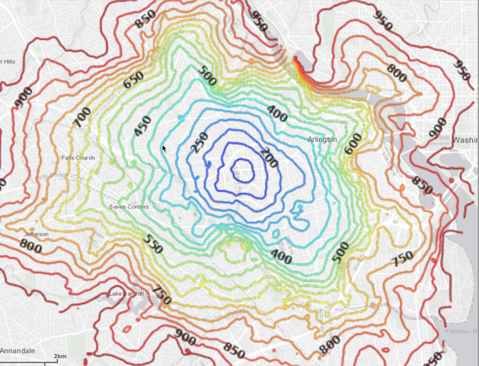
The generated image for Kinetica HQ (leading to) isochrones:

With labels and map data underneath:

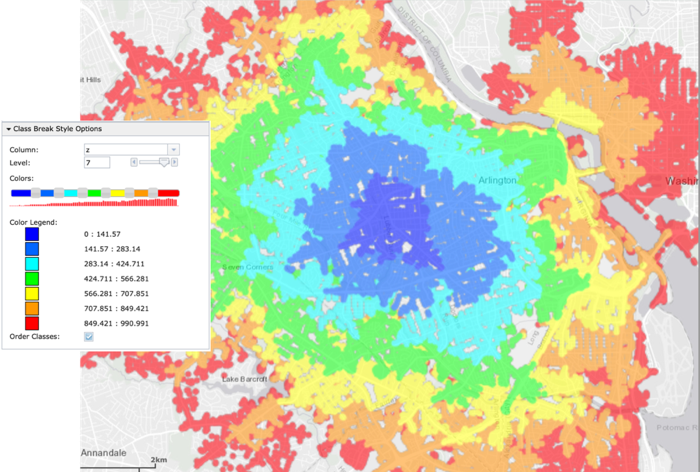
Tip

Using the solve_table (TABLE_K_ISO_SOLVE), you can class break on the z (cost) column in WMS to see individual points and their relative cost:

Download & Run

Included below is a complete example containing all the above requests, the data files, and output.

• Isochrones script
• DC shape data file
• Python output

To run the complete sample, ensure the isochrones.py and dc_shape.csv files are in the same directory (assuming the locations were not changed in the isochrones.py script); then switch to that directory and do the following:

• If on the Kinetica host:

  /opt/gpudb/bin/gpudb_python isochrones.py
  

• If running after using PyPI or GitHub to install the Python API:

  python isochrones.py