Using WKT Data and Geospatial Functions¶

The following sections demonstrate how to ingest and work with WKT data as well as how to use geospatial functions via SQL and the Kinetica Python API. Details about the geospatial functions can be found under Geospatial/Geometry Functions; a list of potential geospatial operations can be found under Geospatial Operations. All geospatial functions are compatible in both native API and SQL expressions.

Prerequisites¶

SQL client configured to use the Kinetica ODBC/JDBC SQL connector
Python API (if running the Python examples)
Sample CSV data files, which should be downloaded & copied to the host running the SQL client. The initialization script references these in the /tmp/data directory, local to where the client is running. If the files are copied to a different directory, the initialization script, geospatial_init.kisql, can be updated accordingly. The data files can be downloaded here:

Loading Sample Data¶

Data loading will be done via the SQL initialization script, which should be run in the SQL client mentioned above.

For instance, if using kisql:

/opt/gpudb/bin/kisql -host localhost < <path/to/scripts/geospatial_init.kisql>

This script will create a collection to house the example tables.

CREATE SCHEMA geospatial_example

A few example tables are created within the collection.

CREATE OR REPLACE REPLICATED TABLE geospatial_example.nyc_neighborhood
(
  gid INT NOT NULL,
  geom WKT NOT NULL,
  CTLabel VARCHAR(16) NOT NULL,
  BoroCode VARCHAR(16) NOT NULL,
  BoroName VARCHAR(16) NOT NULL,
  CT2010 VARCHAR(16) NOT NULL,
  BoroCT2010 VARCHAR(16) NOT NULL,
  CDEligibil VARCHAR(16) NOT NULL,
  NTACode VARCHAR(16) NOT NULL,
  NTAName VARCHAR(64) NOT NULL,
  PUMA VARCHAR(16) NOT NULL,
  Shape_Leng DOUBLE NOT NULL,
  Shape_Area DOUBLE NOT NULL
)

CREATE OR REPLACE REPLICATED TABLE geospatial_example.taxi_trip_data
(
  transaction_id LONG NOT NULL,
  payment_id LONG NOT NULL,
  vendor_id VARCHAR(4) NOT NULL,
  pickup_datetime TYPE_TIMESTAMP,
  dropoff_datetime TYPE_TIMESTAMP,
  passenger_count TINYINT,
  trip_distance REAL,
  pickup_longitude REAL,
  pickup_latitude REAL,
  dropoff_longitude REAL,
  dropoff_latitude REAL
)

CREATE OR REPLACE TABLE geospatial_example.taxi_zone
(
  geom WKT NOT NULL,
  objectid SMALLINT NOT NULL,
  shape_length DOUBLE NOT NULL,
  shape_area DOUBLE NOT NULL,
  zone VARCHAR(64) NOT NULL,
  locationid INT NOT NULL,
  borough VARCHAR(16) NOT NULL,
  PRIMARY KEY (objectid)
)

The data files are used to populate the example tables. The files have a default file path, which can be updated to point to a different valid path on the host running the SQL client if the files were copied to a non-default location:

INSERT INTO nyc_neighborhood
SELECT *
FROM FILE."/tmp/data/nyc_neighborhood.csv"

INSERT INTO taxi_trip_data
SELECT *
FROM FILE."/tmp/data/taxi_trip_data.csv"

INSERT INTO taxi_zone
SELECT *
FROM FILE."/tmp/data/taxi_zone.csv"

Examples via SQL¶

Creating a Table and Inserting WKT Data¶

First, a points-of-interest table is created and loaded with sample WKT data. Per Types, WKT data can be either in byte or string. In the below example, src1_poi and src2_poi are string WKT column type, so the data should be enclosed in quotes.

CREATE OR REPLACE TABLE geospatial_example.points_of_interest
(
  src1_poi WKT NOT NULL,
  src2_poi WKT NOT NULL
)

Then, data is inserted into the WKT table, and the insertion is verified.

INSERT INTO points_of_interest
VALUES
  ('POINT(-73.8455003 40.7577272)','POINT(-73.84550029 40.75772724)'),
  ('POLYGON((-73.9258506 40.8287493, -73.9258292 40.828723, -73.9257795 40.8287387, -73.925801 40.8287635,-73.9258506 40.8287493))','POLYGON((-73.9257795 40.8287387, -73.925801 40.8287635, -73.9258506 40.8287493, -73.9258506 40.8287493,-73.9258292 40.828723))'),
  ('LINESTRING(-73.9942208 40.7504289, -73.993856 40.7500753, -73.9932525 40.7499941)','LINESTRING(-70.9942208 42.7504289, -72.993856 43.7500753, -73.9932525 44.7499941)'),
  ('LINESTRING(-73.9760944 40.6833433, -73.9764404 40.6830626, -73.9763761 40.6828897)','LINESTRING(-70.9761 41.6834, -72.9765 39.6831, -76.9764 38.6829)')

SELECT *
FROM points_of_interest

Scalar Functions¶

For the complete list of scalar functions, see both Scalar Functions and Enhanced Performance Scalar Functions.

Scalar Example 1¶

-- Using GEODIST(), calculate the distance between pickup and dropoff points to
-- see where the calculated distance is less than the recorded trip distance

SELECT *
FROM taxi_trip_data
WHERE GEODIST(pickup_longitude, pickup_latitude, dropoff_longitude, dropoff_latitude) < trip_distance

Scalar Example 2¶

-- Calculate the area of each taxi zone and find the five largest zones

SELECT TOP 5
  objectid AS "Zone_ID",
  zone AS "Zone_Name",
  DECIMAL(ST_AREA(geom, 1) / 1000000) AS "Zone_Area_in_Square_Kilometers"
FROM taxi_zone
ORDER BY 3 DESC

Aggregation Functions¶

For the complete list of aggregation functions, see Aggregation Functions.

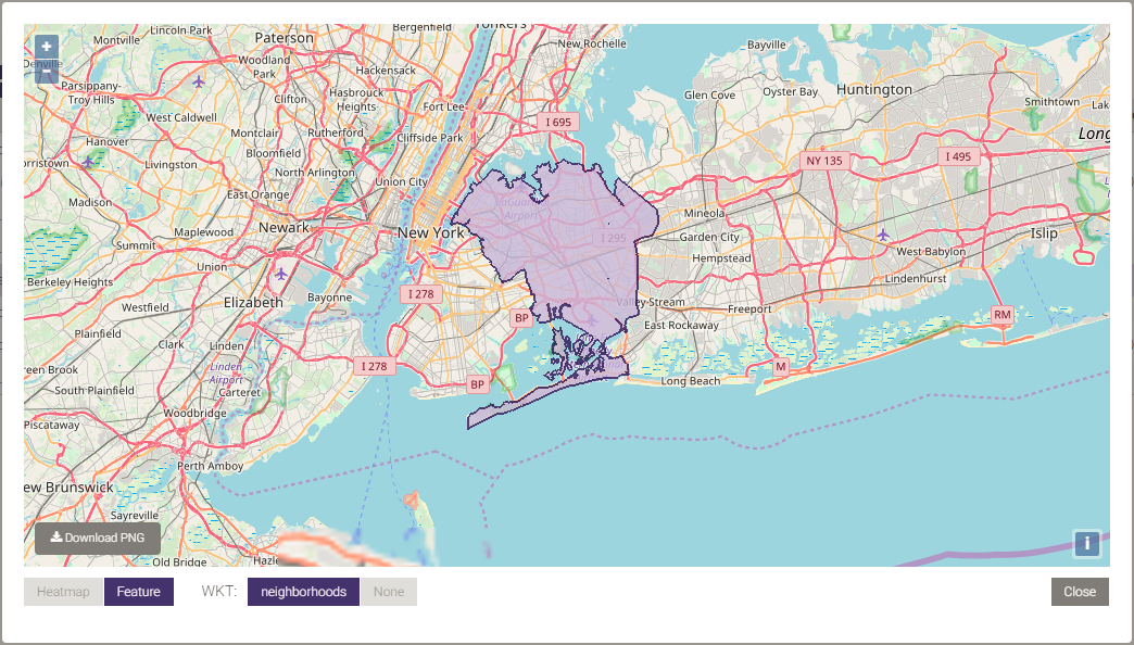
-- Dissolve the boundaries between Queens neighborhood tabulation areas to
-- create a single borough boundary

SELECT
  ST_DISSOLVE(geom) AS neighborhoods
FROM nyc_neighborhood
WHERE BoroName = 'Queens'

Below is a picture of the dissolved neighborhood boundaries:

Joins¶

Many geospatial/geometry functions can be used to join data sets. For the complete list of join and other scalar functions, see both Scalar Functions and Enhanced Performance Scalar Functions.

Join Example 1¶

-- Locate at which borough and neighborhood taxi pickups occurred, and display a
-- subset of those mappings

SELECT TOP 25
  vendor_id AS "Pickup_Vendor_ID",
  passenger_count AS "Total_Passengers",
  pickup_longitude AS "Pickup_Longitude",
  pickup_latitude AS "Pickup_Latitude",
  BoroName AS "Pickup_Borough",
  NTAName AS "Pickup_NTA"
FROM taxi_trip_data, nyc_neighborhood
WHERE STXY_CONTAINS(geom, pickup_longitude, pickup_latitude) = 1

Join Example 2¶

-- Find the top 10 neighborhood pickup locations

SELECT TOP 10
  ntaname AS "Pickup_NTA",
  COUNT(*) AS "Total_Pickups"
FROM
  taxi_trip_data
  JOIN nyc_neighborhood
    ON STXY_Intersects(pickup_longitude, pickup_latitude, geom) = 1
GROUP BY
  ntaname
ORDER BY
  "Total_Pickups" DESC

Join Example 3¶

In some cases, it may be useful to aggregate on the geospatial column itself, applying standard aggregation functions to other joined columns.

-- Find the geospatial objects representing the top 10 neighborhoods,
-- measured by distance covered over all taxi trips originating in them

SELECT TOP 10
  SUM(trip_distance) AS "Total_Trip_Distance",
  geom AS "Pickup_Geo"
FROM
  taxi_trip_data
  JOIN nyc_neighborhood
    ON STXY_Intersects(pickup_longitude, pickup_latitude, geom) = 1
GROUP BY
  geom
ORDER BY
  "Total_Trip_Distance" DESC

Equality¶

There are three ways of checking if two geometries are equal, which each have different thresholds:

ST_EQUALS()
ST_ALMOSTEQUALS()
ST_EQUALSEXACT()

For details on these functions see Scalar Functions.

The data inserted in the first section includes two POINTs that vary slightly in precision, two POLYGONs that vary in the ordering of their boundary points, and two pairs of LINESTRINGs that vary in both precision and scale. Each of these geometry types is compared to see if each given pair is spatially equal as defined by the equality functions:

SELECT
  ST_GEOMETRYTYPE(src1_poi) AS "Source_1_Type",
  ST_GEOMETRYTYPE(src2_poi) AS "Source_2_Type",
  ST_ALMOSTEQUALS(src1_poi, src2_poi, 7) AS "Almost_Equals",
  ST_EQUALS(src1_poi, src2_poi) AS "Equals",
  ST_EQUALSEXACT(src1_poi, src2_poi, 4) AS "Equals_Exact"
FROM points_of_interest
ORDER BY 1

Examples via the Python API¶

Creating a Table and Inserting WKT Data¶

First, a points-of-interest table is created and loaded with sample WKT data. Per Types, WKT data can be either in byte or string. In the below example, src1_poi and src2_poi are string WKT column type, so the data should be enclosed in quotes.

# Create a type using the GPUdbRecordType object
columns = [gpudb.GPUdbRecordColumn("src1_poi", gpudb.GPUdbRecordColumn._ColumnType.STRING,
                                   [gpudb.GPUdbColumnProperty.WKT]),
           gpudb.GPUdbRecordColumn("src2_poi", gpudb.GPUdbRecordColumn._ColumnType.STRING,
                                   [gpudb.GPUdbColumnProperty.WKT])]
poi_record_type = gpudb.GPUdbRecordType(columns, label="poi_record_type")
poi_record_type.create_type(h_db)
poi_type_id = poi_record_type.type_id
# Create a table from the poi_record_type
response = h_db.create_table(table_name=poi_table, type_id=poi_type_id, options={"collection_name": geo_collection})
print "Table created: {}".format(response['status_info']['status'])

Then, data is inserted into the WKT table, and the insertion is verified.

# Prepare the data to be inserted
pois = [
    "POINT(-73.8455003 40.7577272)",
    "POLYGON((-73.9258506 40.8287493, -73.9258292 40.828723, -73.9257795 40.8287387, -73.925801 40.8287635, "
    "-73.9258506 40.8287493))",
    "LINESTRING(-73.9942208 40.7504289, -73.993856 40.7500753, -73.9932525 40.7499941)",
    "LINESTRING(-73.9760944 40.6833433, -73.9764404 40.6830626, -73.9763761 40.6828897)"
]
pois_compare = [
    "POINT(-73.84550029 40.75772724)",
    "POLYGON((-73.9257795 40.8287387, -73.925801 40.8287635, -73.9258506 40.8287493, -73.9258506 40.8287493, "
    "-73.9258292 40.828723))",
    "LINESTRING(-70.9942208 42.7504289, -72.993856 43.7500753, -73.9932525 44.7499941)",
    "LINESTRING(-70.9761 41.6834, -72.9765 39.6831, -76.9764 38.6829)"
]
# Insert the data into the table using a list
encoded_obj_list = []
for val in range(0, 4):
    poi1_val = pois[val]
    poi2_val = pois_compare[val]
    record = gpudb.GPUdbRecord(poi_record_type, [poi1_val, poi2_val])
    encoded_obj_list.append(record.binary_data)
response = h_db.insert_records(table_name=poi_table, data=encoded_obj_list, list_encoding="binary")
print "Number of records inserted:  {}".format(response['count_inserted'])

Scalar Functions¶

For the complete list of scalar functions, see both Scalar Functions and Enhanced Performance Scalar Functions.

Scalar Example 1¶

""" Using GEODIST(), calculate the distance between pickup and dropoff points to see where the calculated distance
    is less than the recorded trip distance """
response = h_db.filter(
        table_name=taxi_trip_table,
        view_name=dist_check_view,
        expression="GEODIST(pickup_longitude, pickup_latitude, dropoff_longitude, dropoff_latitude) "
                    "< trip_distance",
        options={"collection_name": geo_collection}
)
print "Number of trips where geographic distance < recorded distance: {}".format(response["count"])

Scalar Example 2¶

# Calculate the area of each taxi zone and copy the selected data to a projection
h_db.create_projection(
        table_name=taxi_zones_table,
        projection_name=zones_by_area_proj,
        column_names=[
                "objectid", "zone", "ST_AREA(geom,1) / 1000000 AS area"],
        options={"order_by": "area desc", "limit": "5", "collection_name": geo_collection}
)
# Display the top 5 largest taxi zones
large_zones = h_db.get_records(
        table_name=zones_by_area_proj,
        offset=0, limit=gpudb.GPUdb.END_OF_SET,
        encoding="json",
        options={"sort_by":"area", "sort_order": "descending"}
)['records_json']
print "Top 5 largest taxi zones:"
print "{:<7s} {:<27s} {:<30s}".format("Zone_ID", "Zone_Name", "Zone_Area_in_Square_Kilometers")
print "{:=<7s} {:=<27s} {:=<30s}".format("", "", "")
for zone in large_zones:
    print "{objectid:>7d} {zone:<27s} {area:>30.4f}".format(**json.loads(zone))

Aggregation Functions¶

For the complete list of aggregation functions, see Aggregation Functions.

# Dissolve the boundaries between Queens neighborhood tabulation areas to create a single borough boundary
response = h_db.aggregate_group_by(
        table_name=nyc_nta_table,
        column_names=["ST_DISSOLVE(geom) AS neighborhoods"],
        offset=0, limit=1,
        encoding="json",
        options={
                "expression": "BoroName = 'Queens'",
                "result_table": queens_agb,
                "collection_name": geo_collection
        }
)
print "Queens neighborhood boundaries dissolved:  {}".format(response['status_info']['status'])

Below is a picture of the dissolved neighborhood boundaries:

Joins¶

Many geospatial/geometry functions can be used to join data sets. For the complete list of join and other scalar functions, see both Scalar Functions and Enhanced Performance Scalar Functions.

Join Example 1¶

# Locate which borough and neighborhood taxi pickup points occurred
h_db.create_join_table(
        join_table_name=pickup_point_location,
        table_names=[taxi_trip_table + " AS t", nyc_nta_table + " AS n"],
        column_names=[
                "t.vendor_id", "t.passenger_count",
                "t.pickup_longitude", "t.pickup_latitude",
                "n.BoroName", "n.NTAName"
        ],
        expressions=["STXY_CONTAINS(n.geom, t.pickup_longitude, t.pickup_latitude)"],
        options={"collection_name": geo_collection}
)
# Display a subset of the pickup point locations
pickup_points = h_db.get_records(
        table_name=pickup_point_location,
        offset=0, limit=25,
        encoding="json",
        options={"sort_by":"pickup_longitude"}
)['records_json']
print "Subset of pickup point neighborhood locations:"
print "{:<10s} {:<12s} {:<13s} {:<12s} {:<11s} {:<43s}".format("Vendor ID", "Pass. Count", "Pickup Long.",
                                                               "Pickup Lat.", "Borough", "NTA")
print "{:=<10s} {:=<12s} {:=<13s} {:=<12s} {:=<11s} {:=<43s}".format("", "", "", "", "", "")
for point in pickup_points:
    print "{vendor_id:<10s} {passenger_count:<12d} {pickup_longitude:<13f} {pickup_latitude:<12f} "\
          "{BoroName:<11s} {NTAName:<43s}".format(**json.loads(point))

Join Example 2¶

# Find the top neighborhood pickup locations
h_db.create_join_table(
        join_table_name=top_pickup_locations_by_frequency,
        table_names=[taxi_trip_table + " AS t", nyc_nta_table + " AS n"],
        column_names=["n.NTAName AS NTAName"],
        expressions=["((STXY_INTERSECTS(t.pickup_longitude, t.pickup_latitude, n.geom) = 1))"],
        options={"collection_name": geo_collection}
)
# Aggregate the neighborhoods and the count of records per neighborhood
h_db.aggregate_group_by(
        table_name=top_pickup_locations_by_frequency,
        column_names=["NTAName AS Pickup_NTA", "COUNT(*) AS Total_Pickups"],
        offset=0, limit=gpudb.GPUdb.END_OF_SET,
        options={"result_table": pickup_agb, "collection_name": geo_collection}
)
# Display the top 10 neighborhood pickup locations
response = h_db.get_records_by_column(
        table_name=pickup_agb,
        column_names=["Pickup_NTA", "Total_Pickups"],
        offset=0, limit=10,
        encoding="json",
        options={"order_by": "Total_Pickups desc"}
)
data = h_db.parse_dynamic_response(response)['response']
print "Top 10 neighborhood pickup locations:"
print "{:<43s} {:<14s}".format("Pickup NTA", "Total Pickups")
print "{:=<43s} {:=<14s}".format("", "")
for pickupLocs in zip(data["Pickup_NTA"], data["Total_Pickups"]):
    print "{:<43s} {:<14d}".format(*pickupLocs)

Join Example 3¶

In some cases, it may be useful to aggregate on the geospatial column itself, applying standard aggregation functions to other joined columns.

# Find the geospatial objects representing the top 10 neighborhoods by
# distance covered over all taxi trips originating in them
response = h_db.create_join_table(
        join_table_name=top_pickup_locations_by_distance,
        table_names=[taxi_trip_table + " AS t", nyc_nta_table + " AS n"],
        column_names=["n.geom AS geom", "t.trip_distance AS trip_distance"],
        expressions=["((STXY_INTERSECTS(t.pickup_longitude, t.pickup_latitude, n.geom) = 1))"],
        options={"collection_name": geo_collection}
)
# Aggregate the neighborhoods and the count of records per neighborhood
response = h_db.aggregate_group_by(
        table_name=top_pickup_locations_by_distance,
        column_names=["geom AS Pickup_Geo", "SUM(trip_distance) AS Total_Trip_Distance"],
        encoding = "json",
        offset = 0, limit = 10,
        options = {"sort_by":"value", "sort_order":"descending"}
)

Equality¶

There are three ways of checking if two geometries are equal, which each have different thresholds:

ST_EQUALS()
ST_ALMOSTEQUALS()
ST_EQUALSEXACT()

For details on these functions see Scalar Functions.

The data inserted in the first section includes two POINTs that vary slightly in precision, two POLYGONs that vary in the ordering of their boundary points, and two pairs of LINESTRINGs that vary in both precision and scale. Each of these geometry types is compared to see if each given pair is spatially equal as defined by the equality functions:

# Calculate types of geospatial equality for differing sources of geometry
h_db.create_projection(
    table_name=poi_table,
    projection_name=poi_comp_table,
    column_names=[
        "ST_GEOMETRYTYPE(src1_poi) AS src1type",
        "ST_GEOMETRYTYPE(src2_poi) AS src2type",
        "ST_ALMOSTEQUALS(src1_poi, src2_poi, 7) AS almostequals",
        "ST_EQUALS(src1_poi, src2_poi) AS equals",
        "ST_EQUALSEXACT(src1_poi, src2_poi, 4) AS equalsexact"
    ],
    options={"collection_name": geo_collection}
)
equality_comps = h_db.get_records(
        table_name=poi_comp_table,
        offset=0, limit=10,
        encoding="json",
        options={"sort_by":"src1type"}
)['records_json']
print "Comparing ST_ALMOSTEQUALS(), ST_EQUALS(), and ST_EQUALSEXACT():"
print "{:<13s} {:<13s} {:<13s} {:<6s} {:<12s}".format(
        "Source_1_Type", "Source_2_Type", "Almost_Equals", "Equals", "Equals_Exact"
)
print "{:=<13s} {:=<13s} {:=<13s} {:=<6s} {:=<12s}".format("", "", "", "", "")
for comp in equality_comps:
    print "{src1type:<13s} {src2type:<13s} {almostequals:>13d} {equals:>6d} {equalsexact:>12d}".format(**json.loads(comp))

Complete Samples¶

Included below are complete examples containing all the above requests and the output.

Python (see Python Developer Manual for configuration & execution details)
- geospatial_examples.py
- Python Output
SQL (see ODBC/JDBC Connector for configuration & execution details)
- geospatial_examples.kisql
- SQL Output

Table Of Contents

Using WKT Data and Geospatial Functions¶

Prerequisites¶

Loading Sample Data¶

Examples via SQL¶

Creating a Table and Inserting WKT Data¶

Scalar Functions¶

Scalar Example 1¶

Scalar Example 2¶

Aggregation Functions¶

Joins¶

Join Example 1¶

Join Example 2¶

Join Example 3¶

Equality¶

Examples via the Python API¶

Creating a Table and Inserting WKT Data¶

Scalar Functions¶

Scalar Example 1¶

Scalar Example 2¶

Aggregation Functions¶

Joins¶

Join Example 1¶

Join Example 2¶

Join Example 3¶

Equality¶

Complete Samples¶