Solve Graph - Shortest Path with Turn Penalties & Restrictions (DC)

The following is a complete example, using the Python API, of solving a graph created with a Washington, D.C. HERE dataset for a shortest path problem with turn penalties via the /solve/graph endpoint. For more information on Network Graphs & Solvers, see Network Graphs & Solvers Concepts.

Prerequisites

The prerequisites for running this solve graph example are listed below:

• Graph server enabled
• Python API
• Match graph script
• D.C. shape CSV file

Python API Installation

The native Kinetica Python API is accessible through the following means:

• For development on the Kinetica server:
  • Kinetica RPM
• For development not on the Kinetica server:
  • Git
  • PyPI

Kinetica RPM

In default Kinetica installations, the native Python API is located in the /opt/gpudb/api/python directory. The /opt/gpudb/bin/gpudb_python wrapper script is provided, which sets the execution environment appropriately.

Test the installation:

/opt/gpudb/bin/gpudb_python /opt/gpudb/api/python/examples/example.py

Important

When developing on the Kinetica server, use /opt/gpudb/bin/gpudb_python to run Python programs and /opt/gpudb/bin/gpudb_pip to install dependent libraries.

Git

1. In the desired directory, run the following but be sure to replace <kinetica-version> with the name of the installed Kinetica version, e.g., v7.0:

   git clone -b release/<kinetica-version> --single-branch https://github.com/kineticadb/kinetica-api-python.git
   

2. Change directory into the newly downloaded repository:

   cd kinetica-api-python
   

3. In the root directory of the unzipped repository, install the Kinetica API:

   sudo python setup.py install
   

4. Test the installation (Python 2.7 (or greater) is necessary for running the API example):

   python examples/example.py
   

PyPI

The Python package manager, pip, is required to install the API from PyPI.

1. Install the API:

   pip install gpudb --upgrade
   

2. Test the installation:

   python -c "import gpudb;print('Import Successful')"
   

   If Import Successful is displayed, the API has been installed as is ready for use.

Data File

The example script makes reference to a dc_shape.csv data file in the /tmp/data directory. This can be updated to point to a valid path on the host where the file will be located, or the script can be run with the data file in the /tmp/data directory.

CSV = "/tmp/data/dc_shape.csv"

The dc_shape dataset is a HERE dataset and is analogous to most road network datasets you could find in that it includes columns for the type of road, the average speed, the direction of the road, a WKT linestring for its geographic location, a unique ID integer for the road, and more. The graph used in the example is created with four columns from the dc_shape dataset:

• link_id -- a sharded integer column composed of unique IDs for each road segment mapped within this dataset
• shape -- a WKT linestring composed of points that make up various streets, roads, highways, alleyways, and footpaths throughout Washington, D.C.; this column is also part of an inline calculation for distance as weight during graph creation
• direction -- an integer column that conveys information about the directionality of the road, with forward meaning the direction in which the way is drawn in OSM and backward being the opposite direction:
  • 0 -- a forward one-way road
  • 1 -- a two-way road
  • 2 -- a backward one-way road
• speed -- an integer column that represents the average speed travelled on a given road segment; this column is also part of an inline calculation for distance as weight during graph creation

Script Detail

This example is going to demonstrate solving for the shortest path with varying turn-based penalties and restrictions between source points and destination points located within a road network in Washington, D.C.

Constants

Several constants are defined at the beginning of the script:

• TABLE_DC -- the name of the table into which the D.C. road network dataset is loaded
• GRAPH_DC -- the D.C. road network graph
• SOLUTION_GRAPH_DC_1 / SOLUTION_GRAPH_DC_1 / SOLUTION_GRAPH_DC_3 -- the D.C. road network graph shortest path solution tables

TABLE_DC = "dc_shape"
GRAPH_DC = TABLE_DC + "_graph"
SOLUTION_GRAPH_DC_1 = GRAPH_DC + "_solved_sp"
SOLUTION_GRAPH_DC_2 = GRAPH_DC + "_solved_sp_intersection-penalty"
SOLUTION_GRAPH_DC_3 = GRAPH_DC + "_solved_sp_turn-restriction"

Table Setup

Before the graph can be created, the D.C. shape dataset is loaded from a local CSV file. First, the type for this table is first defined:

columns = [
    ["link_id", "long", "shard_key"],
    ["direction", "int"],
    ["speed", "double"],
    ["road_type", "string", "char1"],
    ["seg", "string", "wkt"],
    ["shape", "string", "wkt"],
]

Next, the D.C. shape table is created using the GPUdbTable interface:

t = gpudb.GPUdbTable(
    _type=columns,
    name=TABLE_DC,
    db=kinetica,
    options={}
)

Then the records are created from the CSV file and inserted into the table:

dc_data.next()  # skip the header
records = []
for record in dc_data:
    record_data = [
        int(record[0]),   # link_id
        int(record[1]),   # direction
        float(record[2]), # speed
        record[3],        # road_type
        record[4],        # seg
        record[5]         # shape
    ]
    records.append(record_data)
t.insert_records(records)

Graph Creation

One graph is used for the shortest path solve graph example utilized in the script: GRAPH_DC, a graph based on the dc_shape dataset (the CSV file mentioned in Prerequisites).

The GRAPH_DC graph is created with the following characteristics:

• It is directed because the roads in the graph have directionality (one-way and two-way roads)
• It has no explicitly defined nodes because the example relies on implicit nodes attached to the defined edges
• The edges are derived from WKT LINESTRINGs in the shape column of the dc_shape table (EDGE_WKTLINE). Each road segment's directionality is derived from the direction column of the dc_shape table (EDGE_DIRECTION). Each edge is associated with an ID from the link_id column. Rather than separately define weights, each edge has its weight calculated inline as the length of the entire shape column's LINESTRING (in meters) divided by the number of points in the LINESTRING minus 1 divided by the average speed used to traverse the LINESTRING (EDGE_WEIGHT_VALUESPECIFIED.
• It has no inherent restrictions for any of the edges in the graph
• It utilizes the following options:
  • It will be replaced with this instance of the graph if a graph of the same name exists (recreate)
  • The graph will register dummy edges around each intersection of edges generated from the data to represent turns (add_turns)

cg = kinetica.create_graph(
    graph_name=GRAPH_DC,
    directed_graph=True,
    nodes=[],
    edges=[
        TABLE_DC + ".link_id AS EDGE_ID",
        TABLE_DC + ".shape AS EDGE_WKTLINE",
        TABLE_DC + ".direction AS EDGE_DIRECTION",
        "(ST_LENGTH(" + TABLE_DC + ".shape,1)/"
        "(ST_NPOINTS(" + TABLE_DC + ".shape)-1))/" + 
        TABLE_DC + ".speed AS EDGE_WEIGHT_VALUESPECIFIED"
    ],
    weights=[],
    restrictions=[],
    options={
        "recreate": "true",
        "add_turns": "true"
    }
)

Shortest Path

No Turn Penalties or Restrictions

The first example illustrates a simple shortest path solve from a single source node to a single destination node. First, the source node and destination node are defined.

Note

The source and destination node are the same for each example.

src = ["POINT(-77.04489135742188 38.91112899780273)"]
dest = ["POINT(-77.03193664550781 38.91188049316406)"]

Next, the GRAPH_DC graph is solved with the solve results being exported to the response:

sg = kinetica.solve_graph(
    graph_name=GRAPH_DC,
    solver_type="SHORTEST_PATH",
    source_nodes=src,
    destination_nodes=dest,
    solution_table=SOLUTION_GRAPH_DC_1,
    options={"export_solve_results": "true"}
)["result_per_destination_node"]

The cost for the source node to visit the destination node is represented as time in minutes:

Cost for shortest path between source (['POINT(-77.04489135742188 38.91112899780273)']) and destination (['POINT(-77.03193664550781 38.91188049316406)']):
+---------------------------------------------+---------------------+
| Destination Node                            |   Cost (in minutes) |
+=============================================+=====================+
| POINT(-77.03193664550781 38.91188049316406) |             1.78324 |
+---------------------------------------------+---------------------+

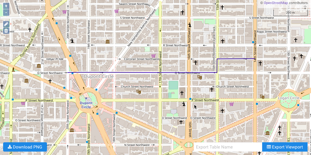
The solution output to WMS:

Intersection Penalty

The second example illustrates a shortest path solve from a single source node to a single destination node, but this time traveling through an intersection of two-way roads will incur an additional cost. The GRAPH_DC graph is solved with the solve results being exported to the response and an intersection penalty of 20 seconds:

sg = kinetica.solve_graph(
    graph_name=GRAPH_DC,
    solver_type="SHORTEST_PATH",
    source_nodes=src,
    destination_nodes=dest,
    solution_table=SOLUTION_GRAPH_DC_2,
    options={
        "export_solve_results": "true",
        "intersection_penalty": "20"
    }
)["result_per_destination_node"]

The cost for the source node to visit the destination node is represented as time in minutes:

Cost for shortest path between source (['POINT(-77.04489135742188 38.91112899780273)']) and destination (['POINT(-77.03193664550781 38.91188049316406)']) with intersection penalty:
+---------------------------------------------+---------------------+
| Destination Node                            |   Cost (in minutes) |
+=============================================+=====================+
| POINT(-77.03193664550781 38.91188049316406) |             2.38018 |
+---------------------------------------------+---------------------+

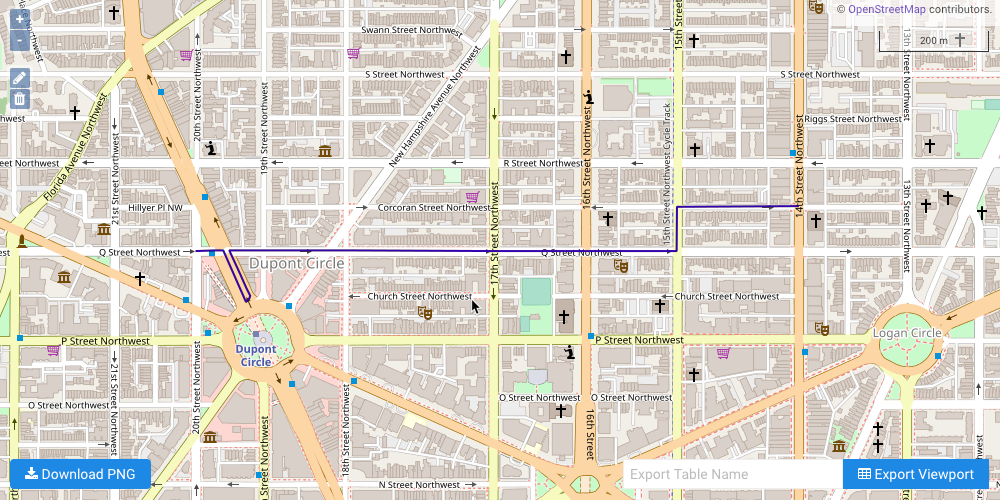
The solution output to WMS, noting the immediate U-turn to return to Q Street from Connecticut Avenue to avoid the intersection penalty:

Turn Restriction

The third example illustrates a shortest path solve from a single source node to a single destination node, but this time a single turn from Q Street on to 15th Street is restricted. The GRAPH_DC graph is solved with turns from road segment ID 18352169 (Q Street) to road segment ID 18352166 (15th Street) being restricted and the solve results being exported to the response:

sg = kinetica.solve_graph(
    graph_name=GRAPH_DC,
    restrictions=[
        "{18352169} AS RESTRICTIONS_FROM_EDGE_ID",
        "{18352166} AS RESTRICTIONS_TO_EDGE_ID",
        "{0} AS RESTRICTIONS_ONOFFCOMPARED"
    ],
    solver_type="SHORTEST_PATH",
    source_nodes=src,
    destination_nodes=dest,
    solution_table=SOLUTION_GRAPH_DC_3,
    options={
        "export_solve_results": "true"
    }
)["result_per_destination_node"]

The cost for the source node to visit the destination node is represented as time in minutes:

Cost for shortest path between source (['POINT(-77.04489135742188 38.91112899780273)']) and destination (['POINT(-77.03193664550781 38.91188049316406)']) with one turn restriction:
+---------------------------------------------+---------------------+
| Destination Node                            |   Cost (in minutes) |
+=============================================+=====================+
| POINT(-77.03193664550781 38.91188049316406) |             2.01081 |
+---------------------------------------------+---------------------+

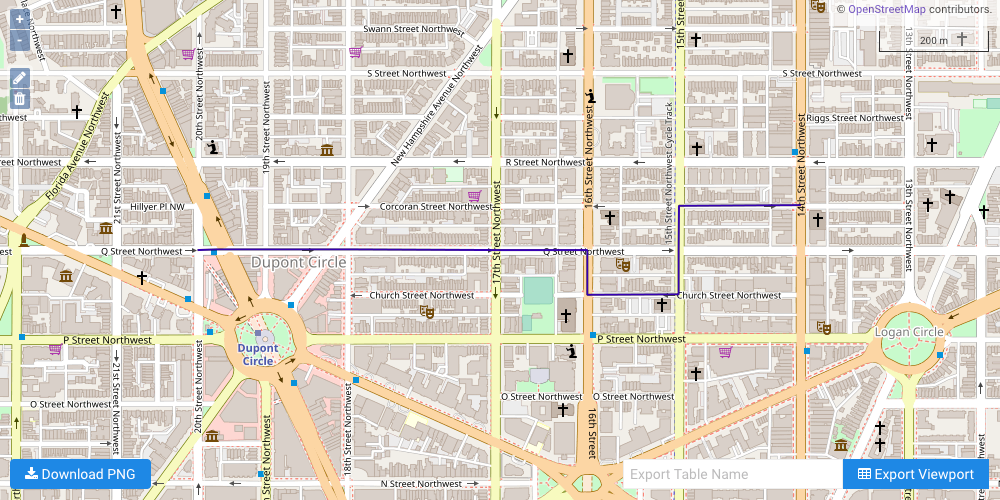
The solution output to WMS, noting the detour on to 16th Street and Church Street to avoid the restricted turn:

Download & Run

Included below is a complete example containing all the above requests, the data files, and output.

• Shortest path solve graph script
• D.C. shape data file
• Python output

To run the complete sample, ensure the solve_graph_dc_shortest_path_turn.py script is in the current directory and the dc_shape.csv file is in the directory defined in that script; then do the following:

• If on the Kinetica host:

  /opt/gpudb/bin/gpudb_python solve_graph_dc_shortest_path_turn.py [--username <username> --password <password>]
  

• If running after using PyPI or GitHub to install the Python API:

  python solve_graph_dc_shortest_path_turn.py [--host <target_host_ip>] [--username <username> --password <password>]