Query Graph - Social (No External Dataset)
The following is a complete example, using the Python API, of querying social relationship data via the /query/graph endpoint. For more information on Network Graphs & Solvers, see Network Graphs & Solvers Concepts.
Prerequisites
The prerequisites for running the query graph example are listed below:
- Kinetica
- Graph server enabled
- Python API
Query graph script
Python API Installation
The native Kinetica Python API is accessible through the following means:
- For development on the Kinetica server:
- For development not on the Kinetica server:
Kinetica RPM
In default Kinetica installations, the native Python API is located in the
/opt/gpudb/api/python directory. The
/opt/gpudb/bin/gpudb_python wrapper script is provided, which sets the
execution environment appropriately.
Test the installation:
/opt/gpudb/bin/gpudb_python /opt/gpudb/api/python/examples/example.py
Important
When developing on the Kinetica server, use /opt/gpudb/bin/gpudb_python to run Python programs and /opt/gpudb/bin/gpudb_pip to install dependent libraries.
Git
In the desired directory, run the following but be sure to replace
<kinetica-version>with the name of the installed Kinetica version, e.g.,v7.0:git clone -b release/<kinetica-version> --single-branch https://github.com/kineticadb/kinetica-api-python.git
Change directory into the newly downloaded repository:
cd kinetica-api-pythonIn the root directory of the unzipped repository, install the Kinetica API:
sudo python setup.py install
Test the installation (Python 2.7 (or greater) is necessary for running the API example):
python examples/example.py
PyPI
The Python package manager, pip, is required to install the API from PyPI.
Install the API:
pip install gpudb --upgrade
Test the installation:
python -c "import gpudb;print('Import Successful')"
If Import Successful is displayed, the API has been installed as is ready for use.
Script Detail
This example is going to demonstrate querying a social network of relationships between friends and family for:
- people directly or indirectly known to a given person who are interested in chess but not known through family
- people directly known to a given gender
- people who are of a given gender or interested in chess
- people directly or indirectly known to a given gender who are interested in chess
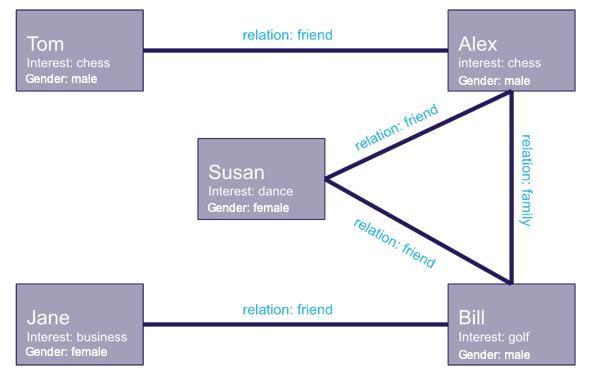
The graph queried in the examples below looks like this:
Constants
Several constants are defined at the beginning of the script:
HOST/PORT-- host and port values for the databaseOPTION_NO_ERROR-- reference to a /clear/table option for ease of use and repeatabilityTABLE_P/TABLE_K-- the names for the tables into which the datasets generated in this file are loaded. These datasets will serve as the basis for the social relationships graph.TABLE_Pis a record of a person's name, age, and interest;TABLE_Kdefines the relationships between the peopleGRAPH_S-- the social relationships graphTABLE_Q1/TABLE_Q2/TABLE_Q3/TABLE_Q4-- the resulting adjacency tables from the four query examples performed in the scriptTABLE_Q1_TARGETS/TABLE_Q2_TARGETS/TABLE_Q3_TARGETS/TABLE_Q4_TARGETS-- the table storing the targets from the first query
HOST = "127.0.0.1"
PORT = "9191"

OPTION_NO_ERROR = {"no_error_if_not_exists": "true"}

TABLE_P = "people"
TABLE_K = "knows"

GRAPH_S = "social_relationships"
TABLE_Q1 = GRAPH_S + "_queried_jane_to_chess"
TABLE_Q2 = GRAPH_S + "_queried_males"
TABLE_Q3 = GRAPH_S + "_queried_females_or_chess"
TABLE_Q4 = GRAPH_S + "_queried_females_to_chess"
TABLE_Q1_TARGETS = TABLE_Q1 + "_targets"
TABLE_Q2_TARGETS = TABLE_Q2 + "_targets"
TABLE_Q3_TARGETS = TABLE_Q3 + "_targets"
TABLE_Q4_TARGETS = TABLE_Q4 + "_targets"
Table Setup
As mentioned previously, there are two tables used in the graph creation step. The first of these tables is the people table. The type for this table is first defined:
p_columns = [
    ["name", "string", "char16"],
    ["age", "int"],
    ["interest", "string", "char16"],
    ["gender", "string", "char8"]
]
Next, the people table is created using the GPUdbTable interface:
table_p_obj = gpudb.GPUdbTable(
    _type=p_columns,
    name=TABLE_P,
    db=kinetica,
    options={}
)
Finally, the people records are defined and inserted:
p_records = [
  ["Susan", 22, "dance", "female"],
  ["Bill", 60, "golf", "male"],
  ["Alex", 34, "chess", "male"],
  ["Jane", 40, "business", "female"],
  ["Tom", 29, "chess", "male"]
]
table_p_obj.insert_records(p_records)
The second table is the knows table. The type for this table is first defined:
k_columns = [
    ["name1", "string", "char16"],
    ["name2", "string", "char16"],
    ["since", "long"],
    ["relation", "string", "char32"]
]
Next, the knows table is created using the GPUdbTable interface:
table_k_obj = gpudb.GPUdbTable(
    _type=k_columns,
    name=TABLE_K,
    db=kinetica,
    options={}
)
Finally, the knows records are defined and inserted:
k_records = [
  ["Jane", "Bill", 2010, "friend"],
  ["Bill", "Susan", 1990, "friend"],
  ["Bill", "Alex", 2001, "family"],
  ["Alex", "Tom", 2001, "friend"],
  ["Susan", "Alex", 2002, "friend"]
]
table_k_obj.insert_records(k_records)
Graph Creation
One graph is used for the query graph example: social_relationships, a graph
based on the people and knows datasets.
The social_relationships graph is created with the following
characteristics:
It is not directed because relationships between people are inherently bi-directional
The people in this graph are represented using
nodesdetailed in thepeopletable: the person's (NODE_NAME), their main interest (NODE_LABEL), and gender (NODE_LABEL).The relationships in this graph are represented using
edgesdetailed in theknowstable: two names to define the relationship (EDGE_NODE1_NAME/EDGE_NODE2_NAME) and the relationship definition (EDGE_LABEL).It has no
weightsbecause this example doesn't favor some relationships over othersIt has no inherent
restrictionsfor any of the nodes or edges in the graphNote
Restrictions will be introduced on a per-query basis later.
It will be replaced with this instance of the graph if a graph of the same name exists (
recreate)
print("Creating {}".format(GRAPH_S))
create_s_graph_response = kinetica.create_graph(
    graph_name=GRAPH_S,
    directed_graph=False,
    nodes = [
      TABLE_P + ".name AS NODE_NAME",
      TABLE_P + ".interest AS NODE_LABEL",
      "",
      TABLE_P + ".name AS NODE_NAME",
      TABLE_P + ".gender AS NODE_LABEL"
    ],
    edges = [
      TABLE_K + ".name1 AS EDGE_NODE1_NAME",
      TABLE_K + ".name2 AS EDGE_NODE2_NAME",
      TABLE_K + ".relation AS EDGE_LABEL"
    ],
    weights = [],
    restrictions = [],
    options={
        "recreate": "true"
    }
)
Querying the Graph
Example 1
To find people interested in chess who are connected to a given person, in this case Jane, in some way (but not through family), we define the graph query in the following way:
- Pass two query identifiers to
queries:- One using
Janeas the name (QUERY_NODE_NAME) of the node from which to begin searching - Pass a blank string (
"") to separate the first query combination from the second - The other using
chessas the label of the target nodes to find (QUERY_TARGET_NODE_LABEL)
- One using
- Use the following restrictions:
- Pass
'family'as the label (RESTRICTIONS_EDGE_LABEL) of the edge in the restriction combination - Pass a
0as an "off" value (RESTRICTIONS_ONOFFCOMPARED) for the edge to set it as restricted
- Pass
- Place the results in
social_relationships_queried_jane_chessadjacency table - Query for nodes within 4 "hops" (
rings) ofJane - Use the options:
- Output the targets found to the
social_relationships_queried_jane_chess_targetstable
- Output the targets found to the
query1_s_graph_response = kinetica.query_graph(
    graph_name=GRAPH_S,
    queries = [
      "{'Jane'} AS QUERY_NODE_NAME",
      "",
      "{'chess'} AS QUERY_TARGET_NODE_LABEL"
    ],
    restrictions = [
      "{'family'} AS RESTRICTIONS_EDGE_LABEL",
      "{0} AS RESTRICTIONS_ONOFFCOMPARED"
    ],
    adjacency_table=TABLE_Q1,
    rings=4,
    options={
      "target_nodes_table": TABLE_Q1_TARGETS
    }
)
The results are retrieved from the social_relationships_queried_jane_chess
adjacency table. The results show two people connected to Jane that are
interested in chess, Alex and Tom. The path to each is listed (represented by
PATH_ID) and the hops to get there (represented by RING_ID). Note that
the PATH_ID and RING_ID data were only available because the
QUERY_TARGET_NODE_LABEL query identifier was used in the query:
+-----------+-----------+--------------------+--------------------+-----------------+
|   PATH_ID |   RING_ID | QUERY_NODE1_NAME   | QUERY_NODE2_NAME   |   QUERY_EDGE_ID |
+===========+===========+====================+====================+=================+
|         2 |         1 | Jane               | Bill               |               1 |
+-----------+-----------+--------------------+--------------------+-----------------+
|         2 |         2 | Bill               | Susan              |               2 |
+-----------+-----------+--------------------+--------------------+-----------------+
|         2 |         3 | Susan              | Alex               |               5 |
+-----------+-----------+--------------------+--------------------+-----------------+
|         3 |         1 | Jane               | Bill               |               1 |
+-----------+-----------+--------------------+--------------------+-----------------+
|         3 |         2 | Bill               | Susan              |               2 |
+-----------+-----------+--------------------+--------------------+-----------------+
|         3 |         3 | Susan              | Alex               |               5 |
+-----------+-----------+--------------------+--------------------+-----------------+
|         3 |         4 | Alex               | Tom                |               4 |
+-----------+-----------+--------------------+--------------------+-----------------+
The targets are retrieved from the
social_relationships_queried_jane_chess_targets table, which shows the
RING_ID, the query sources, and the targets' names, Alex and Tom. The
RING_ID represents the hops required to get from the source to the target.
+-----------+--------------------------+--------------------------+
|   RING_ID | QUERY_NODE_NAME_SOURCE   | QUERY_NODE_NAME_TARGET   |
+===========+==========================+==========================+
|         3 | Jane                     | Alex                     |
+-----------+--------------------------+--------------------------+
|         4 | Jane                     | Tom                      |
+-----------+--------------------------+--------------------------+
Example 2
To find people directly connected to a given gender, in this case male, we define the graph query in the following way:
- Pass a single query to
queriesusingmaleas the label (QUERY_NODE_LABEL) of the node from which to begin searching - Place the results in
social_relationships_queried_malesadjacency table - Use a
ringsvalue of1to only retrieve immediate connections tomales - Use the options:
- Output the targets found to the
social_relationships_queried_male_targetstable
- Output the targets found to the
query2_s_graph_response = kinetica.query_graph(
    graph_name=GRAPH_S,
    queries=[
      "{'male'} AS QUERY_NODE_LABEL"
    ],
    restrictions=[],
    adjacency_table=TABLE_Q2,
    rings=1,
    options={
      "target_nodes_table": TABLE_Q2_TARGETS
    }
)
The results are retrieved from the social_relationships_queried_male
adjacency table. The results show each node within one "hop" of a male node:
+--------------------+--------------------+-----------------+
| QUERY_NODE1_NAME   | QUERY_NODE2_NAME   |   QUERY_EDGE_ID |
+====================+====================+=================+
| Jane               | Bill               |               1 |
+--------------------+--------------------+-----------------+
| Bill               | Susan              |               2 |
+--------------------+--------------------+-----------------+
| Bill               | Alex               |               3 |
+--------------------+--------------------+-----------------+
| Alex               | Tom                |               4 |
+--------------------+--------------------+-----------------+
| Bill               | Alex               |               3 |
+--------------------+--------------------+-----------------+
| Alex               | Tom                |               4 |
+--------------------+--------------------+-----------------+
| Susan              | Alex               |               5 |
+--------------------+--------------------+-----------------+
The targets are retrieved from the social_relationships_queried_males_targets
target nodes table. The results show the name for all nodes that are
connected to the male nodes within one "hop". Duplicate names indicate that
person is within one "hop" of more than one male:
+--------------------------+
| QUERY_NODE_NAME_TARGET   |
+==========================+
| Alex                     |
+--------------------------+
| Susan                    |
+--------------------------+
| Jane                     |
+--------------------------+
| Alex                     |
+--------------------------+
| Susan                    |
+--------------------------+
| Tom                      |
+--------------------------+
| Bill                     |
+--------------------------+
Example 3
To find people who are of a given gender, in this case female, or are interested in chess, we define the graph query in the following way:
- Pass a single query to
queriesusingfemaleandchessas the label (QUERY_NODE_LABEL) of the node for which to search - Place the results in
social_relationships_queried_females_or_chessadjacency table - Use a
ringsvalue of0to only retrieve the nodes that satisfy the query labels - Use the options:
- Output the targets found to the
social_relationships_queried_females_or_chess_targetstable
- Output the targets found to the
query3_s_graph_response = kinetica.query_graph(
    graph_name=GRAPH_S,
    queries=[
      "{'female', 'chess'} AS QUERY_NODE_LABEL",
    ],
    restrictions=[],
    adjacency_table=TABLE_Q3,
    rings=0,
    options={
      "target_nodes_table": TABLE_Q3_TARGETS
    }
)
There are no results in the social_relationships_queried_females_or_chess
because the rings value was set to 0, meaning there will be no
adjacencies.
The targets are retrieved from the
social_relationships_queried_females_or_chess_targets target nodes table.
The results show the name for the nodes that are female or interested in chess:
+--------------------------+
| QUERY_NODE_NAME_TARGET   |
+==========================+
| Alex                     |
+--------------------------+
| Tom                      |
+--------------------------+
| Jane                     |
+--------------------------+
| Susan                    |
+--------------------------+
Example 4
To find people directly or indirectly known to a given gender who are interested in chess, we define the graph query in the following way:
- Pass two query identifiers to
queries:- One using
femaleas the label (QUERY_NODE_LABEL) of the node from which to begin searching - Pass a blank string (
"") to separate the first query combination from the second - The other using
chessas the label of the target nodes to find (QUERY_TARGET_NODE_LABEL)
- One using
- Place the results in
social_relationships_queried_females_to_chessadjacency table - Use a
ringsvalue of2to find nodes within two "hops" of the female nodes - Use the options:
- Output the targets found to the
social_relationships_queried_females_to_chess_targetstable
- Output the targets found to the
query4_s_graph_response = kinetica.query_graph(
    graph_name=GRAPH_S,
    queries=[
        "{'female'} AS QUERY_NODE_LABEL",
        "",
        "{'chess'} AS QUERY_TARGET_NODE_LABEL"
    ],
    restrictions=[],
    adjacency_table=TABLE_Q4,
    rings=2,
    options={
      "target_nodes_table": TABLE_Q4_TARGETS
    }
)
The results are retrieved from the
social_relationships_queried_females_to_chess adjacency table. The results
show two females, Susan and Jane, connected (within two "hops") to two people
that are interested in chess, Alex and Tom. The path to each is listed
(represented by PATH_ID) and the hops to get there (represented by
RING_ID). Note that the PATH_ID and RING_ID data were only
available because the QUERY_TARGET_NODE_LABEL query identifier was used in
the query:
+-----------+-----------+--------------------+--------------------+-----------------+
|   PATH_ID |   RING_ID | QUERY_NODE1_NAME   | QUERY_NODE2_NAME   |   QUERY_EDGE_ID |
+===========+===========+====================+====================+=================+
|         3 |         1 | Jane               | Bill               |               1 |
+-----------+-----------+--------------------+--------------------+-----------------+
|         3 |         2 | Bill               | Alex               |               3 |
+-----------+-----------+--------------------+--------------------+-----------------+
|         2 |         1 | Susan              | Alex               |               5 |
+-----------+-----------+--------------------+--------------------+-----------------+
|         3 |         1 | Susan              | Alex               |               5 |
+-----------+-----------+--------------------+--------------------+-----------------+
|         3 |         2 | Alex               | Tom                |               4 |
+-----------+-----------+--------------------+--------------------+-----------------+
The targets are retrieved from the
social_relationships_queried_females_to_chess target nodes table. The
results show the name for the nodes that are interested in chess and the "hops"
required to get there:
+-----------+--------------------------+--------------------------+
|   RING_ID | QUERY_NODE_NAME_SOURCE   | QUERY_NODE_NAME_TARGET   |
+===========+==========================+==========================+
|         2 | Jane                     | Alex                     |
+-----------+--------------------------+--------------------------+
|         1 | Susan                    | Alex                     |
+-----------+--------------------------+--------------------------+
|         2 | Susan                    | Tom                      |
+-----------+--------------------------+--------------------------+
Download & Run
Included below is a complete example containing all the above requests, the data files, and output.
To run the complete sample, switch to the directory in which the
query_graph_social.py is located, then do the following:
If on the Kinetica host:
/opt/gpudb/bin/gpudb_python query_graph_social.py
If running after using PyPI or GitHub to install the Python API:
python query_graph_social.py