Solve Graph - Backhaul (Seattle)

The following is a complete example, using the Python API, of solving a graph created with Seattle road network data for a backhaul routing problem via the /solve/graph endpoint. For more information on Network Graphs & Solvers, see Network Graphs & Solvers Concepts.

Prerequisites

The prerequisites for running the backhaul routing solve graph example are listed below:

• Kinetica (v. 7.0 or later)
• Graph server enabled
• Python API
• Solve graph script
• Seattle road network CSV file

Python API Installation

The native Kinetica Python API is accessible through the following means:

• For development on the Kinetica server:
  • Kinetica RPM
• For development not on the Kinetica server:
  • Git
  • PyPI

Kinetica RPM

In default Kinetica installations, the native Python API is located in the /opt/gpudb/api/python directory. The /opt/gpudb/bin/gpudb_python wrapper script is provided, which sets the execution environment appropriately.

Test the installation:

/opt/gpudb/bin/gpudb_python /opt/gpudb/api/python/examples/example.py

Important

When developing on the Kinetica server, use /opt/gpudb/bin/gpudb_python to run Python programs and /opt/gpudb/bin/gpudb_pip to install dependent libraries.

Git

1. In the desired directory, run the following but be sure to replace <kinetica-version> with the name of the installed Kinetica version, e.g., v7.0:

   git clone -b release/<kinetica-version> --single-branch https://github.com/kineticadb/kinetica-api-python.git
   

2. Change directory into the newly downloaded repository:

   cd kinetica-api-python
   

3. In the root directory of the unzipped repository, install the Kinetica API:

   sudo python setup.py install
   

4. Test the installation (Python 2.7 (or greater) is necessary for running the API example):

   python examples/example.py
   

PyPI

The Python package manager, pip, is required to install the API from PyPI.

1. Install the API:

   pip install gpudb --upgrade
   

2. Test the installation:

   python -c "import gpudb;print('Import Successful')"
   

   If Import Successful is displayed, the API has been installed as is ready for use.

Data File

The example script makes reference to a road_weights.csv data file in the current directory. This can be updated to point to a valid path on the host where the file will be located, or the script can be run with the data file in the current directory.

CSV = "road_weights.csv"

Script Detail

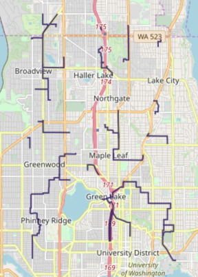
This example is going to demonstrate solving for routing a given set of remote assets, e.g., stores, to a number of fixed assets, e.g, distribution centers, located in a Seattle road network.

Constants

• HOST / PORT -- host and port values for the database
• OPTION_NO_ERROR -- reference to a /clear/table option for ease of use and repeatability
• TABLE_SRN -- the name of the table into which the Seattle road network dataset is loaded
• GRAPH_S -- the Seattle road network graph
• GRAPH_S_BSOLVED -- the solved Seattle road network graph using the BACKHAUL_ROUTING solver type

HOST = "127.0.0.1"
PORT = "9191"

OPTION_NO_ERROR = {"no_error_if_not_exists": "true"}

TABLE_SRN = "seattle_road_network"

GRAPH_S = TABLE_SRN + "_graph"
GRAPH_S_BSOLVED = GRAPH_S + "_backhaul_routing_solved"

Graph Creation

One graph is used for the backhaul solve graph example utilized in the script: seattle_road_network_graph, a graph based on the road_weights dataset (the CSV file mentioned in Prerequisites).

The seattle_road_network_graph graph is created with the following characteristics:

• It is directed because the roads in the graph have directionality (one-way and two-way roads)
• It has no explicitly defined nodes because the example relies on implicit nodes attached to the defined edges
• The edges are represented using WKT LINESTRINGs in the WKTLINE column of the seattle_road_network table (EDGE_WKTLINE). The road segments' directionality is derived from the TwoWay column of the road_weights table (EDGE_DIRECTION).
• The weights are represented using the time taken to travel the segment found in the time column of the seattle_road_network table (WEIGHTS_VALUESPECIFIED). The weights are matched to the edges using the same WKTLINE column as edges (WEIGHTS_EDGE_WKTLINE) and the same TwoWay column as the edge direction (WEIGHTS_EDGE_DIRECTION).
• It has no inherent restrictions for any of the nodes or edges in the graph
• It will be replaced with this instance of the graph if a graph of the same name exists (recreate)

print("Creating {}".format(GRAPH_S))
create_s_graph_response = kinetica.create_graph(
    graph_name=GRAPH_S,
    directed_graph=True,
    nodes=[],
    edges=[
        TABLE_SRN + ".WKTLINE AS EDGE_WKTLINE",
        TABLE_SRN + ".TwoWay AS EDGE_DIRECTION"
    ],
    weights=[
        TABLE_SRN + ".WKTLINE AS WEIGHTS_EDGE_WKTLINE",
        TABLE_SRN + ".TwoWay AS WEIGHTS_EDGE_DIRECTION",
        TABLE_SRN + ".time AS WEIGHTS_VALUESPECIFIED"
    ],
    restrictions=[],
    options={
        "recreate": "true"
    }
)

Backhaul Routing

First, the fixed assets and remote assets are set.

fixed_assets = [
    "POINT(-122.37694377950754 47.69058183874783)",
    "POINT(-122.37591381124582 47.6947415132984)",
    "POINT(-122.3635541921052 47.70005617015495)",
    "POINT(-122.35565776876535 47.70583235665686)",
    "POINT(-122.35531444601145 47.72477375603093)",
    "POINT(-122.33540172628489 47.72361898977214)",
    "POINT(-122.32407207540598 47.72408089934756)",
    "POINT(-122.32647533468332 47.73562730759159)",
    "POINT(-122.32922191671457 47.74209217807247)",
    "POINT(-122.31205577901926 47.741399551774876)",
    "POINT(-122.31274242452707 47.737705389219734)",
    "POINT(-122.29935283712473 47.73701270455902)",
    "POINT(-122.2976362233552 47.73262548770682)",
    "POINT(-122.2921430592927 47.73354914302527)",
    "POINT(-122.29179973653879 47.72200227400312)",
    "POINT(-122.30003948263254 47.712531931184785)",
    "POINT(-122.30278606466379 47.701442513285734)",
    "POINT(-122.30518932394114 47.694048257248284)",
    "POINT(-122.30244274190989 47.68827076507089)",
    "POINT(-122.31514568380442 47.68480396253861)",
    "POINT(-122.32750530294504 47.68711518982914)",
    "POINT(-122.3474180226716 47.687577422998146)",
    "POINT(-122.37763042501535 47.686421832395006)",
    "POINT(-122.37694377950754 47.69058183874783)"
]
remote_assets = [
    "POINT(-122.324612 47.725231)", "POINT(-122.362112 47.696131)",
    "POINT(-122.356212 47.74173099999999)", "POINT(-122.341512 47.702631)",
    "POINT(-122.327412 47.737131)", "POINT(-122.344912 47.727531)",
    "POINT(-122.291612 47.65763099999999)", "POINT(-122.324512 47.703831)",
    "POINT(-122.297712 47.731231)", "POINT(-122.317912 47.699431)",
    "POINT(-122.351412 47.713731)", "POINT(-122.295612 47.670531)",
    "POINT(-122.321812 47.672731)", "POINT(-122.295612 47.697531)",
    "POINT(-122.333012 47.689831)", "POINT(-122.298812 47.711731)",
    "POINT(-122.309612 47.684931)", "POINT(-122.359712 47.716431)",
    "POINT(-122.360612 47.659231)", "POINT(-122.299012 47.707431)",
    "POINT(-122.311612 47.66683099999999)", "POINT(-122.315912 47.724631)",
    "POINT(-122.316912 47.709531)", "POINT(-122.313212 47.685731)",
    "POINT(-122.321712 47.721231)", "POINT(-122.339512 47.695031)",
    "POINT(-122.310512 47.692531)", "POINT(-122.326512 47.679731)",
    "POINT(-122.358112 47.705731)", "POINT(-122.352812 47.715931)",
    "POINT(-122.291612 47.67753099999999)", "POINT(-122.295712 47.666731)",
    "POINT(-122.303712 47.681531)", "POINT(-122.362312 47.732231)",
    "POINT(-122.347712 47.740431)", "POINT(-122.343512 47.68523099999999)",
    "POINT(-122.326412 47.730631)", "POINT(-122.357812 47.67003099999999)",
    "POINT(-122.321012 47.694531)", "POINT(-122.353312 47.737131)",
    "POINT(-122.323412 47.67903099999999)", "POINT(-122.351012 47.701731)",
    "POINT(-122.349112 47.735931)", "POINT(-122.361612 47.675031)",
    "POINT(-122.320912 47.70193099999999)", "POINT(-122.345412 47.693331)",
    "POINT(-122.357112 47.669631)", "POINT(-122.352912 47.685131)",
    "POINT(-122.361712 47.681331)", "POINT(-122.346312 47.722231)"
]

Next, the graph is solved with the solve results being exported to the response. The fixed assets are provided for the source nodes and the remote assets are provided for the destination nodes:

solve_s_bgraph_response = kinetica.solve_graph(
    graph_name=GRAPH_S,
    solver_type="BACKHAUL_ROUTING",
    source_nodes=fixed_assets,
    destination_nodes=remote_assets,
    solution_table=GRAPH_S_BSOLVED,
    options={"export_solve_results": "true"}
)["result_per_destination_node"]

The cost for each remote to travel to the nearest fixed asset is output:

Cost for each remote asset to travel to nearest fixed asset:
Remote Asset                           Cost (in minutes)
=====================================  =================
POINT(-122.324612 47.725231)           0.865516
POINT(-122.362112 47.696131)           0.758842
POINT(-122.356212 47.74173099999999)   1.084458
POINT(-122.341512 47.702631)           1.246927
POINT(-122.327412 47.737131)           0.263679
POINT(-122.344912 47.727531)           0.730477
POINT(-122.291612 47.65763099999999)   2.255474
POINT(-122.324512 47.703831)           1.546832
POINT(-122.297712 47.731231)           0.761547
POINT(-122.317912 47.699431)           1.088295
POINT(-122.351412 47.713731)           0.781952
POINT(-122.295612 47.670531)           1.331788
POINT(-122.321812 47.672731)           2.004906
POINT(-122.295612 47.697531)           1.966542
POINT(-122.333012 47.689831)           1.346219
POINT(-122.298812 47.711731)           0.349077
POINT(-122.309612 47.684931)           0.431795
POINT(-122.359712 47.716431)           0.822105
POINT(-122.360612 47.659231)           2.150527
POINT(-122.299012 47.707431)           0.845038
POINT(-122.311612 47.66683099999999)   2.345284
POINT(-122.315912 47.724631)           2.599283
POINT(-122.316912 47.709531)           1.695174
POINT(-122.313212 47.685731)           0.251388
POINT(-122.321712 47.721231)           0.786522
POINT(-122.339512 47.695031)           1.121402
POINT(-122.310512 47.692531)           0.724923
POINT(-122.326512 47.679731)           0.452152
POINT(-122.358112 47.705731)           0.461203
POINT(-122.352812 47.715931)           1.164492
POINT(-122.291612 47.67753099999999)   2.552220
POINT(-122.295712 47.666731)           2.504816
POINT(-122.303712 47.681531)           1.311244
POINT(-122.362312 47.732231)           1.250877
POINT(-122.347712 47.740431)           0.588394
POINT(-122.343512 47.68523099999999)   1.167451
POINT(-122.326412 47.730631)           1.249203
POINT(-122.357812 47.67003099999999)   1.425482
POINT(-122.321012 47.694531)           1.741059
POINT(-122.353312 47.737131)           1.464322
POINT(-122.323412 47.67903099999999)   1.690359
POINT(-122.351012 47.701731)           0.978331
POINT(-122.349112 47.735931)           0.652920
POINT(-122.361612 47.675031)           1.161741
POINT(-122.320912 47.70193099999999)   0.810048
POINT(-122.345412 47.693331)           1.174176
POINT(-122.357112 47.669631)           0.283823
POINT(-122.352912 47.685131)           1.114293
POINT(-122.361712 47.681331)           1.756808
POINT(-122.346312 47.722231)           1.190125

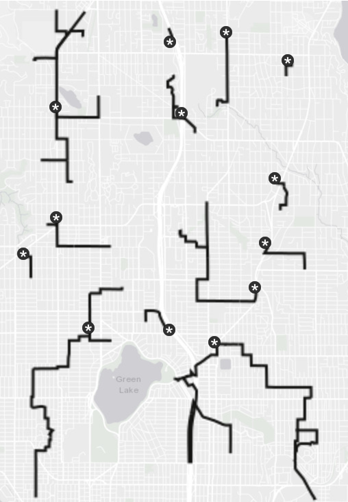
The solution output to WMS:

Tip

To demonstrate how the remote assets are routed back to the fixed assets, the fixed assets can be plotted using a separate WMS call and mapped together with the solution. The picture below represents this; the fixed assets are * icons while remote assets can be found in lines leading away from the fixed assets.

Download & Run

Included below is a complete example containing all the above requests, the data files, and output.

• Backhaul routing solve graph script
• Seattle road network data file
• Python output

To run the complete sample, ensure the solve_graph_seattle_backhaul.py and road_weights.csv files are in the same directory (assuming the locations were not changed in the solve_graph_seattle_backhaul.py script); then switch to that directory and do the following:

• If on the Kinetica host:

  /opt/gpudb/bin/gpudb_python solve_graph_seattle_backhaul.py
  

• If running after using PyPI or GitHub to install the Python API:

  python solve_graph_seattle_backhaul.py